
1. Introduction
Identifying asset price bubbles is a prime concern for achieving financial and macroeconomic stability. Therefore, detecting asset price bubbles in financial and macroeconomic time series data has become a significant area of research in economics. An asset price bubble forms when the valuation of an asset exceeds its fundamental value (Stiglitz, 1990). Financial, commodity, and derivatives markets can be seriously affected by these bubbles. Recent crises such as the 1990 Dotcom bubble and the 2007 global financial crisis have shown the detrimental effect that a bubble in one market can disseminate across other markets. A plethora of literature has been developed to propose or improve the theoretical and statistical modelling of asset price bubbles (Allen et al., 2006; Barassi et al., 2020; Gomez-Gonzalez et al., 2017; LeRoy & Porter, 1981; Shiller, 1981; and Galí et al., 2021).
A major challenge in econometric identification is assessing prices in relation to fundamentals, which requires the measurement of fundamentals. We assume that the actual price or price-dividend ratio consists of both fundamental and non-fundamental components. One solution to address this challenge is to estimate the fundamental component from an underlying structural relationship involving measurable variables. Existing methods often use the actual price or price-dividend ratio with dividends as proxies for fundamentals (Blanchard, 1979; Diba & Grossman, 1988; Evans, 1991). The popularity of this solution is mostly due to its convenience. However, these methods are not perfect, as detection tests mainly identify the primary time series characteristics of the bubble component, which is only partially present in asset prices or log PD ratios.
To improve bubble detection, it is essential to decompose the asset price into fundamental and non-fundamental components. Phillips et al. (2021) used a reduced-form IVX-AR model for this purpose, while others have applied various decomposition methods (Anderson & Brooks, 2014; Campbell et al., 2009; Gordon, 1959; Hafsal & Durai, 2020, p. 2022; Lee, 1995). This paper proposes a new alternative method, unexplored in the current literature, to detect asset price bubbles by identifying a better market fundamental, which is easy for academics and practitioners to use. By identifying the fair fundamental, investors can make more informed decisions, potentially enhancing portfolio construction and investment strategies. This approach allows investors to focus on the intrinsic value of assets, reducing the risk of investing in overinflated stocks during bubble periods.
This study explores a new method to assess the fundamental value of stocks’ market prices without using external variables. It examines whether minimizing the cross-sectional variance and skewness of index components can help identify market bubbles. This method decomposes market prices into fundamental components and bubble components. The study’s contribution lies in using cross-sectional information from a stock index to identify bubbles, unlike most other studies that focus only on time-series analysis.
Very few studies talk about the importance of cross-sectional information in understanding asset price movements (McEnally & Todd, 1992) and its relationship with speculative bubbles (Anderson & Brooks, 2014). The proposed method’s basis is backed by the theoretical framework to understand the transitory deviation of inflation from the underlying trend emanating from firms’ cross-sectional behavior to the price change, as specified in Ball & Mankiw (1994) (BM hereafter). Deriving a similar parlance, the component stocks that constitute the market index react to their fundamentals, like firms’ reactions to a price change in the BM model. If the skewness of the price change of individual/firm return component stocks is considered an aggregate shock, minimizing the skewness will give us the fundamental return of the market index. Following the model explained in the next section, it involves three steps: the first step is to have the time series of the market index, and its component stock prices, with weights aggregating to the market index over time. Second, the skewness of the distribution of the cross-sectional return of component stocks is minimized every period to derive the fundamental return of the market return. Third, convert this identified fundamental return to derive the fundamental market price, with the remaining term being bubbles.
To our knowledge, no other research employs the information on the cross-sectional moments of the stock returns that constitute the market index to derive fundamental and bubble values. The existing approach to fundamental extraction relies on a function of different economic variables. The market fundamental which we derive is directly extracted from the stocks, rather than depending on other variables. This helps us clearly extract the fundamentals. Most importantly, merely mapping the price-dividend ratio or any other ratios to stock prices will not give much insight into market movements, as many markets do not regularly distribute dividends. Our new approach provides a valid alternative to understanding market movements using price itself.
II. Methodology
The new approach follows Ball & Mankiw’s (1994) theoretical framework and the empirical framework of Rather et al. (2016). In a traditional present value model, the price of an asset Pt contains the fundamental component, Ft, and a bubble component, Bt, as A stock price’s fair or fundamental value can be identified by subtracting the transitory or bubble part from the actual price. To derive the fundamental value, we modify the model of Ball & Mankiw (1994) in the stock market context.
Consider a market that contains several sectors, each with a set of imperfectly competitive firms, and their stocks are traded in the market. The expected price change (return) of a firm’s stock equals +θ, where is the fundamental price change common across all the stocks in the sector and θ is a non-fundamental idiosyncratic shock that follows skewed normal distribution f(θ) with 0 mean probability density function. In the presence of asymmetric information and investor behaviour, not all the firms in the sector and not all sectors in the market get equal attention. With a transaction cost, C, that follows a cumulative distribution function G(.), the actual price change of a sector is and the realized aggregate return of the market is as follows:
ΔPm= ΔPf+∫ꝏ−ꝏθG(|θ|) f(θ)d(θ)
Hence, if the density of the transitory shock f(θ) is symmetric then the actual price change is the same as However, if f(θ) is asymmetric and skewed then the actual price change differs from Based on this argument, we minimize the skewness of the actual price to reduce the influence of on and uncover a common component of price change that is the same across all the stocks, which we term the market’s fundamental return. To minimize the skewness, we adopt the method introduced by Rather et al. (2016) as follows:
-
Calculate the change in the price (ΔPit) of the ith stock for period t as ln(Pit/Pit-1); hence the market return is defined as: ΔPt=N∑i=1wiΔPit where N represents the total number of stocks and represents the weight assigned for the ith stock.
-
Organize each stock price change, ΔPit, in ascending or descending order with their concerned weights for each period.
-
A grid-search method is applied to determine the range of stock price changes {i*, j*} which minimizes the absolute skewness |Sh |. The search method can be written as follows: Sh=(∑jh=iwh(ΔPh−ΔP)3)× (∑jh=iwh)1/2(∑jh=iwh(ΔPh−ΔP)2)3/2 For all j = {n, n-1, n-2….T}, i = {1, 2, 3,….j-T+1}, where T is the upper limit that leaves minimum required data for the estimation of skewness, and ΔP is the sample mean of price change in each period. For each period, this produces estimate of skewness for every time period.
-
The fundamental return of the market for period t, specified as the weighted average of stock price changes within the optimal range i* to j*, is calculated as:
Pft=j∗∑h=i∗whPh/j∗∑h=i∗wh
This method’s advantage is that the trimming range, which could be symmetric or asymmetric for each period, is endogenously and uniquely determined based on the size and sign of skewness.
III. Data
The data used to implement this new approach are monthly data of all the 30 stocks included in the Dow Jones Industrial Average (DJIA) Index of the US from May 1994 to May 2019. Since the DJIA Index is an equally weighted index with a base divisor, the study provides equal weights to all stocks with an appropriate base divisor. The data on all the 30 individual stocks included in the Dow Jones Index and the market index are obtained from the Yahoo Finance website at www.finance.yahoo.com.
IV. Empirical Results
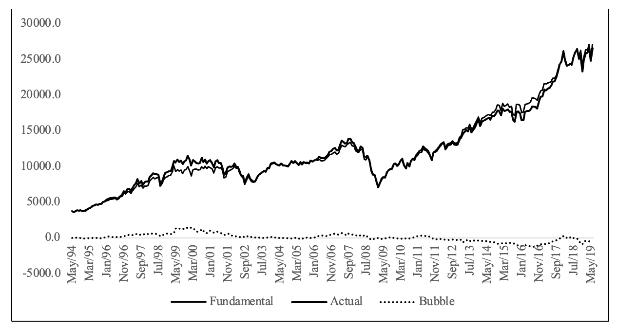
This study detects bubbles by minimizing the skewness of the cross-sectional returns of stocks in the DJIA index. The minimum skewness range and its weighted value for each period are treated as the market’s fundamental return, with the rest considered the bubble component.

From the figure, we can infer that the fundamental follows the actual price most of the period except in some periods. During the 1998-2002 period, it shows that the actual price deviates from the fundamental value, indicating the bubble’s presence during that period. During this period, the bubble can be explained by the now-famous Dotcom bubble of IT companies in the US, indicating that the Dotcom bubble relates to the NASDAQ market and its consequences spread across the DJIA index too (Brunnermeier & Nagel, 2004; Smith & Smith, 2005). Another major deviation of actual price from its fundamental was during the period from 2006 onwards, demonstrating the existence of bubbles in the market. The projected fundamental value using our method during this period is remarkably lower than the actual price and corresponds to the global financial crisis. The new alternate approach identifies the bubbles consistent with the US economy’s specific events and the market.

To evaluate this model’s validity, we compare the results with a recent study by Siess (2019), based on the two-scale LPPL method. The result produced in this study is precisely similar to that of Siess (2019), which involves complex computation. Figure 2 illustrates the two-stage LPPM model of the DJIA index. The figure depicts that the black line represents the actual DJIA index, and the continuous red line corresponds to the two-scale LPPL formula, while the red dashed line corresponds to its main macroscopic component. He studied the DJIA index from 1988 to 2019 and clearly identified the Dotcom bubble of 1998-2000 and the Global Financial Crisis of 2006-2008, which is the same as what we found in our approach. Calibrating the two-stage LPPM formula with respect to a given time series is not as easy as it may seem. Even though the number of parameters is small, the function to optimize may exhibit a great number of local minima, rendering the optimization a little risky.
The advantage of the proposed new methodology over his approach is that it distinguishes the price into a fundamental component and bubble component and extracts it over the sample period. Furthermore, the decomposed components can be used to understand their usefulness in various financial applications, including portfolio optimization.
V. Conclusion
This paper proposes a new approach to understanding asset price bubbles by identifying market fundamentals. Our method uses cross-sectional asset returns to identify these fundamentals, differing from existing methods. Applied to the DJIA index, our method effectively extracts fundamental and bubble components, identifying bubble episodes such as the Dotcom bubble and the 2007-08 financial crisis. The simplicity of our method allows investors to use the extracted fundamental and bubble values in their investment strategies, though it does not determine the fundamental values of individual series.