

I. Introduction
Understanding exchange rate volatility is important to devise and design policies aimed at maintaining macroeconomic stability—an important ingredient for investments and economic growth. The literature (see, Balg & Metcalf, 2010; Cevik et al., 2017; Devereux & Lane, 2003) on exchange rate volatility, particularly, what determines it, is voluminous. This literature can be categorized into various strands. Prominent amongst these are theoretical models of Devereux and Lane (2003) which see a role for external financial liabilities. On the empirical side, focus has been on explaining exchange rate volatility due to stock return volatility (Kanas, 2022), soft power variables, such as index of voice and accountability, life expectancy, education, banking sector fragility, financial openness, and the role of agriculture (Cevik et al., 2017), and macroeconomic volatility (Balg & Metcalf, 2010).
A subset of the literature to which our note connects to is about the effect of interventions to control exchange rate volatility. In this scholarship, interventions have taken different meanings. Glick et al (1995) and Glick and Wihlborg (1997), for instance, proxy intervention with the percentage change in international reserves as a fraction of the monetary base while Bayoumi and Eichengreen (1998) proxy intervention with the percentage change in narrow money. They find that interventions are important influences of exchange rate volatility.
We depart from the standard approaches to defining intervention and consider direct regulator intervention in controlling prices. In Fiji, the Fijian Competition and Consumer Commission (FCCC) is the price regulator. Over the sample period we consider, there were 59 months in which price control measures were implemented. This represents almost 50% of the months in which prices were regulated. Our hypothesis is that FCCC’s price intervention strategy by having a positive effect on domestic prices helps reduce Fiji’s nominal exchange rate volatility. Using time series regression models, we unravel strong evidence that FCCC’s price control strategy reduces exchange rate volatility: every intervention reduced volatility by around 3.5%. Ours is the first paper that models the specific role of a price regulator in achieving exchange rate stability. Our proposed approaches and models can be used to study other country cases to develop a consensus on the effectiveness of price regulator.
II. Motivation and Preliminaries
In Figure 1 we plot Fiji’s nominal exchange rate, which is monthly and for the period January 2011 to March 2022. The rate is quoted in terms of Fiji Dollar (FJD) per United States Dollar (USD) such that an increase in the rate represents a depreciation of the FJD. A number of features are worth highlighting. First, the mean exchange rate over the sample is 2.013, that is, on average one USD buys 2.013 FJD. The rate was recorded lowest (1.734) in August 2011 and was at its weakes in March 2022, when one USD bought 2.33 FJD.

The rate’s standard deviation stands at 0.15%. A first order autoregressive model estimated using the ordinary least squares recorded a slope coefficient of 0.99 and a t-statistic of 62.65, suggesting a very high level of persistence. We conducted a test for the order of integration. In doing so, given the evidence of structural breaks in Figure 1, we employ the Narayan and Popp (2010, 2013) two endogenous structural break unit root test. We allow for two breaks in levels of the data, allow for a maximum of 4 lags (and optimize lag length using the Schwarz information criterion), and use a trimming factor of 10% (given the small sample size we have, a 10% trimming factor is sufficient). The resulting break dates are January 2017 and August 2018—both are statistically different from zero (with a t-statistic > 4).
The t-statistic for the unit root null hypothesis is -4.955 and with a 5% significance level critical value of -4.514, we reject the null hypothesis of a unit root. This implies that Fiji’s nominal exchange rate is structural break stationary in levels.
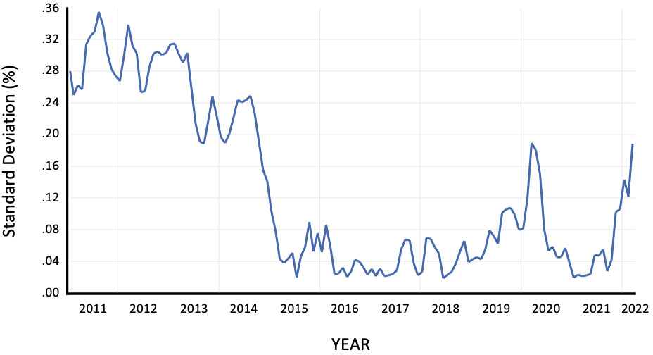
We then run a generalized autoregressive conditional heteroskedasticity (GARCH) model with a lag structure for ARCH and GARCH terms set to 1. We assume a normal error distribution given that descriptive statistics test on normality based on the Jarque-Bera test confirmed that the nominal exchange rate was normal. The mean equation runs the nominal rate on a constant and extracts the conditional standard deviation, which we use as a proxy for exchange rate volatility. This volatility occupies Figure 2. We see that the volatility of Fiji’s nominal exchange rate has declined substantially from 2014 onwards. Between 2015 to 2020, the volatility has been well contained and has been stable. Post-2020, marked by the COVID-19 pandemic, we see higher volatility in the nominal exchange rate.
A feature of pricing data in Fiji is that the FCCC has been prominent in price regulations, aimed at maximizing consumer and producer welfare. Has this contributed to this smoothening of exchange rate volatility?
III. Econometric Framework and results
To test our hypothesis, we propose the following time-series regression model:
NERt=∝+β1FCCCt+β2FCCCt−1+β3FCCCt−2+eNER,t
Equation (1) depicts the relationship between Fiji’s nominal exchange rate (NER) and the price regulations imposed by FCCC, which takes a dummy variable representation with a value one in months of price control and zero in the rest of the months. The regression is estimated using ordinary least squares.
The regression results are tabulated below (see Table 1). This table reports results from four different models. Model A is the base model that regresses the exchange rate volatility on FCCC’s price control intervention. Model B explores how effective FCCC’s price control works on the nominal exchange rate volatility two months after the price control. Models C and D augment Model B with two control variables, oil price and consumer price inflation. The regression is estimated using ordinary least squares and the proxy for exchange rate volatility is its conditional standard deviation extracted from a GARCH (1,1) model with Gaussian error distribution.
We start we a variant of Equation (1) that tests only the contemporaneous effect of FCCC’s price regulation on nominal exchange rate. The following results are obtained: The basic model suggests that FCCC’s price control intervention reduces exchange rate volatility by 3.3%–that is, every month of FCCC’s intervention volatility falls by 3.3%, which in Model B improves to a reduction in volatility by 3.5% when lag effects of FCCC’s effectiveness is considered. When specific control variables are included in Models C and D, the month of intervention effect remains robust at 3.5%. The results reveal that the impact of FCCC’s price controls stays in the exchange rate market for up to two months; that is, the FCCC intervention is found to be statistically significant for up to two months.
IV. Concluding Remarks
The objective of this note was to investigate the effect of FCCC’s price control measures on the volatility of Fiji’s nominal exchange rate. We utilize a GARCH model to extract the volatility of the nominal exchange rate; we employ the unconditional GARCH-based standard deviation as our proxy for exchange rate volatility. Fitting a time-series regression model of FCCC’s price control intervention on Fiji’s nominal exchange rate, we find that each month of FCCC’s intervention reduces volatility by between 3.3% to 3.5% and we find that the impact of this intervention lasts for two months in the exchange rate market.
These finding masks the key role played by FCCC as a price regulator in Fiji’s economic progress. Exchange rate is a fundamental macroeconomic variable of interest to policy makers and investors alike. While the effectiveness of FCCC’s role as a regulator of prices on reducing exchange rate volatility is confirmed by our study, future discussions should focus on how this role can be enhanced.