A Liquidity Mismatch Index (LMI) for Indian Banks

I. Introduction

The global financial crisis underscored how liquidity stress rather than solvency issues alone can trigger systemic instability in banking systems. In response, Basel III introduced regulatory tools such as the iquidity coverage ratio (LCR) and the net stable funding ratio (NSFR), which have since been widely adopted, including in India (Bhuyan & Srimany, 2014). However, these measures are largely static and rule-based, lacking a strong theoretical foundation and often failing to capture the dynamic interaction between asset liquidity and liability structure during periods of stress (Bai et al., 2018). To address these limitations, the liquidity mismatch index (LMI) was proposed as a more flexible and forward-looking alternative by Bai et al. (2018). The LMI integrates balance sheet data with time-varying liquidity weights on both assets and liabilities, offering a dynamic perspective on liquidity risk.

While the LMI has gained traction in advanced economies, its empirical application in emerging markets remains limited. In particular, little is known about how liquidity mismatches vary across bank ownership structures, such as between state-owned and domestic private banks, or how systemic events like the COVID-19 pandemic influence these dynamics. These questions are especially relevant in the Indian context, where the banking sector is characterized by diverse ownership structures and significant differences in regulatory treatment, governance, and market access (Acharya, 2012). Given these institutional characteristics, an LMI-based assessment can provide deeper insight into the vulnerabilities of Indian banks under stress.

This paper contributes by reviewing the conceptual framework and construction of the LMI and applying it to Indian banks over the period 2011–2022. It addresses three key research questions: (i) How has the LMI evolved over time? (ii) Does the extent of liquidity mismatch differ between state-owned and private banks? and (iii) What is the impact of COVID-19 on these mismatches? In doing so, the study builds on the broader literature on liquidity creation and systemic risk (Berger & Bouwman, 2009; Brunnermeier & Pedersen, 2009; Kladakis et al., 2022), empirical liquidity assessments (Chung et al., 2018), critiques of static regulatory tools (Chiaramonte & Casu, 2017; Wei et al., 2017), and recent extensions of the LMI framework (Legroux et al., 2022; Roberts et al., 2018). In addition to tracking the evolution of LMI across Indian banks, the paper offers ownership-specific insights into liquidity behavior showing that state-owned banks tend to exhibit higher mismatches than private counterparts. It further explores whether banks facing higher liability-side pressures actively adjust their asset-side buffers, shedding light on liquidity management strategies. By incorporating the COVID-19 shock into the analysis, the paper also illustrates the LMI’s responsiveness to real-time financial disruptions. These contributions provide useful inputs for improving liquidity monitoring frameworks and designing forward-looking macroprudential policies in emerging market contexts.

The remainder of the paper proceeds as follows: Section II outlines the LMI construction methodology, Section III presents the empirical findings, and Section IV concludes with policy implications.

II. Evolution of Liquidity Assessment

Two primary forms of liquidity risk exist: market liquidity risk, which pertains to the challenges of converting non-cash assets into cash, and funding liquidity risk, which refers to the ability to meet liquid obligations as they come due (Brunnermeier & Pedersen, 2009). An analysis of 900 banks across 29 countries indicates that institutions may need to utilize near-cash assets when deposit run-offs exceed 10 percent to cover the shortfall (IMF, 2023).

Numerous recent studies have concentrated on liquidity. Notably, Berger and Bouwman (2009) developed measures illustrating the amount of liquidity created by banks. These measures have been adopted in various research efforts (Kladakis et al., 2022). Other scholars (Chung et al., 2018) have also calculated different liquidity metrics. Concurrently, the Basel Committee has proposed several liquidity ratios, although their effectiveness remains debated (Chiaramonte & Casu, 2017; Wei et al., 2017).

In this context, the Liquidity Mismatch Index has emerged as a valuable alternative. Bai et al. (2018) note that the LMI “measures the mismatch between the market liquidity of assets and the funding liquidity of liabilities” (pp.52). To date, only a limited number of studies have thoroughly examined the utility of this measure, predominantly within advanced economies (Legroux et al., 2022; Roberts et al., 2018).

III. Liquidity Mismatch Index (LMI)

The calculation of the LMI is based on the following assumptions. First, creditors aim to extract the maximum amount of cash from the bank according to the agreed terms and conditions, defining the liability side liquidity. Second, the bank uses its balance sheet to generate as much cash as possible to meet immediate liquidity outflows, defining the asset side liquidity. The LMI is determined as the net difference between liability-side and asset-side liquidity. Analytically, the LMI for bank $b$ at time $t$ is defined as:

$${LMI}_{t}^{b} = \sum_{k}^{\mathstrut}{\lambda_{t,A_{k}}A_{t,k}^{b}} + \sum_{k}^{\mathstrut}{\lambda_{t,L_{k}}L_{t,k}^{b}} \tag{1}$$

In Equation (1), $A$ and $L$ show the value of asset and liabilities of type k for bank b and $\lambda_{t}$ are the corresponding asset- and liability-side liquidity weights. Operationally, the liquidity weights are defined as:

$$\lambda_{t,A_{k}}^{b} = 1 - m_{t,k} \tag{2}$$

$$\lambda_{t,L_{k}}^{b} = {- exp}(µ_{t}T_{k}) \tag{3}$$

In Equation (2), m is the haircut (ranging from zero to one) on asset of type k, with those having greater ease of liquidation having lower haircuts. Therefore, the product of the asset category with the haircut provides overall market liquidity. In Equation (3), $µ$ captures the expected duration of the stress event (higher values indicating shorter duration) and $T$ is the maturity profile of the liability. It is measured as [$- \alpha\ ln(OIS - Tbill)$], where $\alpha$ is a non-negative parameter and $OIS$ denotes overnight index swap.^[1] More liquid liabilities receive lower maturity, based on the conjecture that these funds will be the one to be encashed the earliest during a liquidity stress.

IV. Data and Evolution of LMI

We use balance sheet and market-related data for an unbalanced panel of 45 domestic Indian banks from 2011 to 2022, yielding 488 bank-year observations. All variables are adjusted to reduce the impact of outliers beyond the 1st and 99th percentiles.

The financial variables include Tobin’s Q and the spread between the 3-month OIS rate and the 91-day Treasury bill yield, representing short-term market liquidity conditions. Tobin’s Q is calculated using market value data obtained from the Prowess database, while the OIS and T-bill yields are sourced from the Bloomberg terminal. The liquidity weights—defined as haircuts on assets and maturities on liabilities—follow the framework proposed by Bai et al. (2018) and are summarized in Table 1.

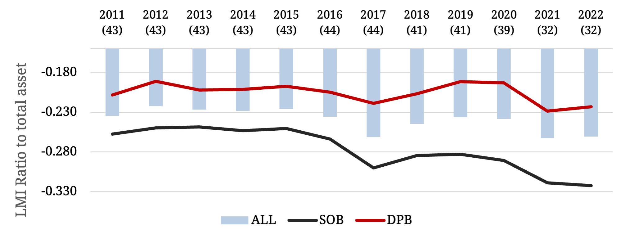
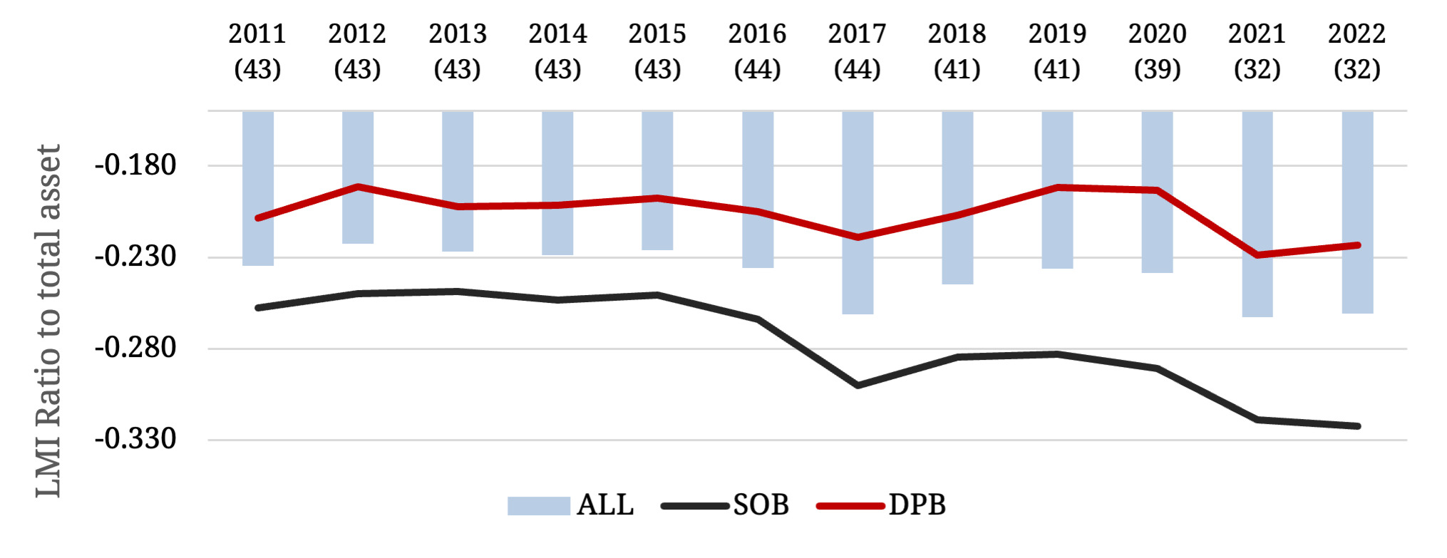
Figure 1 presents the time-series evolution of the LMI, disaggregated by bank ownership and year. The number of banks included in each year decreases over time, reflecting consolidation and mergers within the banking sector. Figure 1 reveals that, on average, state-ownedbank (SOBs) exhibit higher liquidity mismatches than domestic private banks (DPBs). A plausible explanation is that SOBs benefit from an implicit government guarantee, allowing them to tolerate greater mismatches without immediate market penalty (Acharya, 2012). The visual findings from Figure 1 are further substantiated by empirical analysis in the subsequent section.

Figure 1.LMI by bank ownership and year

Source: Author’s calculations Note: Here, SOB denotes state-owned bank, DPB denotes domestic private bank and ALL denotes the total of SOB and DPB

V. Methodology and Results

To investigate the link between asset- and liability-side liquidity, akin to Bai et al. (2018), for bank b at year t we utilise the following specification:

$$\begin{aligned} {ALQ\ (asset)}_{bt} &= {\theta\ Abs.\left\lbrack LLQ\ (liab.) \right\rbrack}_{bt}\\ & \quad + \beta\ {Controls}_{bt} + \lambda\ {Merger}_{bq}\\ & \quad + {fixed\ effects}_{b} + {fixed\ effects}_{t}\\ & \quad + \varepsilon_{bt} \end{aligned}\tag{4}$$

where the response variable is asset-side LMI (as ratio to total asset). On the RHS, the key coefficient is $\theta$, which shows the response of the liability-side (Table 2 provides the variable definitions).

Theoretically, funding shortfalls during stress periods would compel banks to liquidate non-cash assets (after exhausting cash and equivalents), thereby reducing their market liquidity. This value degradation is perceived as a credit-negative by the market, creating a feedback loop (“liquidity spirals”) between market and funding liquidity. Consequently, banks with higher potential liquidity pressure on the liability side may seek to hold more liquidity on the asset side to cover for such exigencies, so that $\theta > 0$. The specification also includes bank-specific controls (Controls). Standard errors are clustered by bank. Results are presented in Table 3.

In column 1, θ is negative and statistically significant with a point estimate of -0.19. As a result, banks facing higher liability-side liquidity challenges do not mitigate them by holding additional assets. The point estimate suggests that banks might deliberately adopt such a strategy (a fully unmatched position would entail a coefficient of -1). An increase in liability-side LMI by one standard deviation reduces asset-side liquidity by approximately 0.7 percent on average.

Next, we include the bank-specific controls, continuing to find evidence supporting that liability-side liquidity pressures do not have a discernible impact on asset-side LMI. In column 3, we explore the relevance of COVID-19 in this relationship by including the interaction of the absolute value of LMI and COVID as an additional regression. The evidence clearly shows that COVID-19 exacerbated the liquidity mismatch. Using the point estimates, a one standard deviation increase in liability-side LMI in the presence of COVID reduced asset-side LMI by nearly 2 percent.

It is possible that the results are susceptible to inter-group heteroscedasticity or even intra-group autocorrelation and inter-group contemporaneous correlation. We address this challenge by estimating the model using the Feasible Generalized Least Squares (FGLS) technique (Xu et al., 2022). Even then, the key coefficients remain unchanged in sign and significance (column 4).

We examine the response separately for SOBs in column 5 and DPBs in column 6. The liability-side responsiveness to the asset-side is driven primarily by SOBs. The evidence also indicates that the impact of COVID-19 on liability-side LMI was much larger for SOBs. Taken together, this suggests that banks have a significant liquidity mismatch on their balance sheets which is not counterbalanced by asset-side liquidity.

The control variables indicate that larger and well-capitalized banks maintain higher asset-wide liquidity mismatches, contrary to findings reported elsewhere (Bai et al., 2018; Legroux et al., 2022). This phenomenon is observed mainly for state-owned banks (column 4), whereas for private banks (column 5), high growth opportunities and lower management inefficiencies drive them to enhance market liquidity.

VI. Conclusion

Two policy recommendations are proposed. First, it would be beneficial to supplement regulatory-prescribed liquidity measures with LMI that can provide insights into liquidity behavior, particularly during periods of stress. Second, stress periods can result in asset firesales. In this context, the LMI adds dynamism to static models by indicating the extent to which cash equivalents can mitigate stress arising from funding liquidity.

The analysis has several limitations. Firstly, the time-varying weights in the LMI can be challenging to calculate accurately, especially during stress periods. Secondly, SOBs often have additional layers of government guarantees, which might not be readily available to their private counterparts. A comprehensive assessment of these underlying nuances in the context of LMI could be valuable for future research.