The Role of Corruption in Shaping Environmental Quality in India: A Quantile Regression Approach

I. Introduction

Corruption is a widespread issue that infiltrates the economy, significantly impacting economic development, governance, and environmental quality. It is a challenge that affects countries of all sizes and income levels, creating inefficiencies and exacerbating inequalities. The World Bank (1997) defines corruption as “the misuse of public office for private gain.” According to the World Economic Forum (2012), the global cost of corruption is estimated to be around US$2.6 trillion, accounting for nearly 5% of the world’s GDP. The study of corruption has gained momentum in recent years, with extensive research examining its causes and consequences across nations (Elbahnasawy & Revier, 2012). Importantly, corruption is not only an economic deterrent but also a crucial determinant of ecological deterioration (Sadiq et al., 2024).

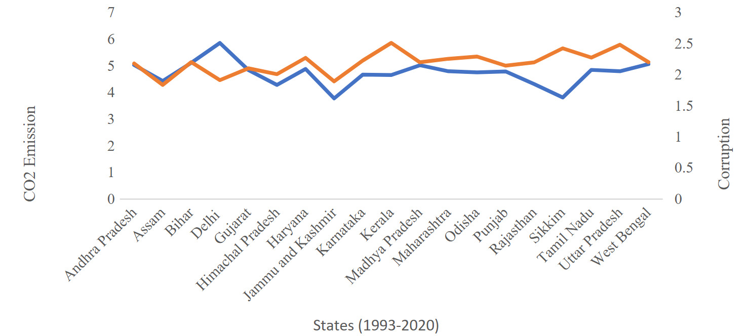
In recent years, climate change and carbon emissions have taken centre stage in global policy discussions, with international agreements such as the Paris Agreement. The United Nations Sustainable Development Goals (SDGs) have also highlighted climate action as a priority, recognising the need for institutional reforms to address environmental challenges. Research suggests that institutional quality, especially corruption, significantly influences environmental outcomes. It weakens regulatory enforcement, undermines environmental policies, and enables polluters to evade compliance, thereby increasing carbon emissions and environmental degradation (Candau & Dienesch, 2017; Dincer & Fredriksson, 2018). Through bribery and rent-seeking, firms circumvent environmental regulations, diminishing incentives for cleaner production and reducing policy effectiveness. The Indian context provides a compelling case for examining the corruption-environment nexus. As one of the world’s largest and fastest-growing economies, India faces severe environmental challenges, including deteriorating air quality, deforestation, and rising CO₂ emissions. According to the Global Carbon Atlas, India was the third-largest emitter of CO₂ in 2020, with emissions driven by rapid urbanisation, industrialisation, and reliance on fossil fuels. At the same time, corruption remains a significant governance issue at both the national and state levels. Previous literature has explored the nexus between corruption and environmental standards, often highlighting an inverse correlation. Lisciandra and Migliardo (2007) provided empirical evidence that corruption directly reduces environmental quality by allowing polluters to bypass regulations. Similarly, Sinha et al. (2019) demonstrated that corruption hampers the effectiveness of environmental policies, resulting in increased emissions and pollution-related health burdens. Figure 1 shows the trend in average CO₂ emissions and corruption across Indian states from 1993–2020.

Figure 1.Average CO₂ emission and corruption across Indian States (1993-2020)

Despite the growing body of literature on corruption and environmental quality, only a few studies have examined how corruption affects sub-national CO₂ emissions in India. Given the significant variation in both corruption levels and environmental policies across Indian states, a state-wise analysis can provide valuable insights into the mechanisms through which corruption influences carbon emissions. This research seeks to address this gap by studying the causality between corruption and CO₂ emissions across Indian states from 1993 to 2020. Additionally, it examines how corruption interacts with CO₂ emissions in different quantiles, thereby contributing to the broader discourse on governance and environmental sustainability. By analysing the state-level variations, this study offers policy-relevant insights into how corruption affects environmental outcomes in India. Understanding this relationship is crucial for designing more effective anti-corruption measures and environmental policies that can mitigate CO₂ emissions.

The rest of this paper is organised as follows: The study’s data and methods are presented in Section II, the empirical findings are discussed in Section III, and the conclusion is provided in Section IV.

II. Data and Methodology

The Corruption Index (CORR) was constructed using conviction cases reported in the Crimes in India report, published by the Government of India. Specifically, the number of conviction cases registered under the Prevention of Corruption Act, 1988, along with relevant penal codes, was utilised to develop the CORR. This study analyses data from 18 states^[1] and the Union Territory of Delhi over the period 1993–2020. State-wise carbon dioxide (CO₂) emissions and energy consumption (ENG) data were sourced from the Global Data Lab, while real per capita income (GDP) and urbanisation (URB) figures were obtained from CMIE States. Additionally, data on state government expenditure (GOV) as a percentage of GDP were extracted from CMIE States. Regional financial development (FND) was measured as the ratio of private credit outstanding to nominal SGDP, with data sourced from the RBI database. Information on the regional industrial structure (IND) was also gathered from the RBI database. The baseline model is represented by Equation (1).

$$\begin{aligned}{CO2}_{it} =& \beta_{it} + \beta_{2t}{CORR}_{it} + \beta_{3t}{GDP}_{it} + \beta_{4t}{ENG}_{it} \\&+ \beta_{5t}{FND}_{it} + \beta_{6t}{GOV}_{it} + \beta_{7t}{IND}_{it} \\&+ \beta_{8t}{URB}_{it} + \mu_{it}\end{aligned}\tag{1}$$

The study utilises the method of moments quantile regression (MMQR) due to its advantages over traditional quantile regression. MMQR extends conventional quantile regression by incorporating moment conditions to account for unobserved heterogeneity and distributional effects across different quantiles of the dependent variable. Unlike standard quantile regression (SQR), which assumes that covariates affect only the location of the conditional distribution, MMQR allows for both location and scale shifts, making it more flexible in capturing heterogeneous relationships. The SQR model does not account for potential unobserved heterogeneity within panel data. However, MMQR introduces fixed effects and considers distributional changes beyond just the mean and median effects (Machado & Silva, 2019).

III. Results

Table 1 presents descriptive statistics for 19 Indian states from 1993 to 2020. The average CO₂ emissions is 4.72, ranging from 3.51 to 6.00. The CORR index has a mean of 1.39, indicating moderate variation across states. GDP and ENG have mean values of 4.62 and 2.65, respectively. FND and GOV average 1.41 and 1.07, reflecting disparities among states. URB shows a negative mean of -0.58, while IND averages 1.46 with low dispersion. Overall, the data reveal considerable economic, institutional, and environmental variation across the states.

The MMQR regression analysis results are presented in Table 2 (and Figure A presented in the Appendix), providing insights into the determinants of CO₂ emissions across different quantiles. The findings indicate a positive and statistically significant relationship between corruption and CO₂ emissions across all quantiles. This supports the institutional quality hypothesis, which suggests that weak governance and corruption can lead to ineffective environmental regulations, increased illegal industrial activities, and excessive exploitation of resources, further exacerbating emissions (Cole, 2007; Khan & Hassan, 2024). Economic growth exhibits a strong positive impact on CO₂ emissions at lower quantiles, with its effect declining at higher quantiles. This finding supports the Environmental Kuznets Curve (EKC) hypothesis, which posits that the early stages of economic and industrial growth lead to increased emissions; however, as economies develop and adopt cleaner technology, emissions decline (Acheampong, 2018; Kaika & Zervas, 2013).

The impact of energy consumption on CO₂ emissions is nonlinear across different quantiles. At lower quantiles, energy consumption has a positive effect, indicating that in the early stages of economic development, higher energy demand is met through increased CO₂ emissions (Acheampong, 2018; Sadorsky, 2009). However, at higher quantiles, energy consumption exerts a negative effect on emissions. This suggests that as growth accelerates, economies undergo structural transformations characterised by greater investments in cleaner energy sources, technological innovations, and stringent environmental policies. These developments contribute to improved energy efficiency and a gradual transition towards renewable energy (Ang, 2007; Sadorsky, 2009; Yuan et al., 2014).

The results show a negative and significant effect of financial development on CO₂ emissions, particularly at higher quantiles. This finding is supported by the “green finance” hypothesis, which suggests that well-developed financial markets facilitate investments in clean energy and environmentally sustainable projects, thereby reducing emissions (Lv & Li, 2021; Shahbaz et al., 2013). Government expenditure decreases CO₂ emissions considerably at lower quantiles, demonstrating the efficacy of environmental regulations, green subsidies, and renewable energy initiatives. However, this effect diminishes at higher quantiles, where economies are more carbon-intensive and structural reliance on fossil fuels limits policy efficacy. This indicates that, although government actions help to reduce emissions initially, further steps are required for long-term reductions in high-emission economies (Fan et al., 2020; Halkos & Paizanos, 2013).

Across all quantiles, industrial activity significantly lowers CO₂ emissions. While this may appear contradictory, it can be explained by the structural transformation theory, which holds that states with developed industrial structures reduce their carbon footprint by transitioning towards more technologically advanced and energy-efficient industries (Chang, 2015). Moreover at higher quantiles, where rapid urban growth fuels increased energy use, transportation emissions, and industrial activity, urbanisation dramatically increases CO₂ emissions. Emissions rise as cities expand due to the increasing need for infrastructure, transportation, and power, which increases dependency on fossil fuels (Wang et al., 2014). To mitigate the negative effects of urbanisation on the environment, this underscores the importance of energy-efficient technologies, greener transportation systems, and sustainable urban design.

To further strengthen the main regression results, we have used the adjusted corruption index^[2] as a robustness measure for the conviction of corruption. Table 3 (and Figure B given in the Appendix) present the results of the robustness test. The findings confirm that the main results remain robust when the adjusted corruption index is used.

IV. Conclusion

The study finds that higher levels of corruption significantly increase CO₂ emissions across Indian states, emphasising the need for governance reforms to achieve sustainability goals. Moreover, strengthening institutional mechanisms through independent environmental ombudsman offices can enhance enforcement and curb rent-seeking behaviour. In addition, improving transparency through digital emission monitoring and public disclosure can increase accountability and trust. Furthermore, linking fiscal incentives to environmental performance can motivate states to adopt cleaner technologies and responsible governance. These measures can align anti-corruption initiatives with sustainable and low-carbon development.