Impact of Climate Change on Inflation and Output in Indonesia

I. Introduction

Climate change (CC) has emerged as one of the most severe challenges faced by both global economies and individual countries. CC poses risks related to extreme weather conditions such as irregular rainfall, droughts, floods, rising sea levels, and ever-increasing temperatures, all of which directly threaten economic activities and macroeconomic stability (OECD, 2015). The Bank of England (BoE, 2022) noted that CC influences both the supply and demand sides of the macroeconomy. Thus, recognizing these potential disruptions and analyzing the impact of CC in a macroeconomic context has become crucial. Consequently, researchers have increasingly begun to examine the implications of CC for macroeconomic outcomes.

There is a growing body of literature analyzing the impact of CC on macroeconomic variables (Mukherjee & Ouattara, 2021). Much of this research is driven by the need to assess both the direct and indirect effects of climate change on inflation, output growth, and overall macroeconomic stability (BoE, 2022). This makes the issue particularly relevant for central banks, as climate-related risks are becoming an integral part of monetary and financial stability frameworks (BoE, 2022). Furthermore, it is argued that developing and emerging market economies (EMEs) are often more vulnerable to CC shocks due to their structural characteristics and limited adaptive capacity. Thus, it is important to explore the impact of CC from the perspective of EMEs.

Based on the above research issues, it becomes vital to analyze the macroeconomic implications of climate change in the context of EMEs. Thus, the objective of this study is to examine the impact of climate change on inflation and output growth in an emerging economy, Indonesia. We select Indonesia as it is an island-based economy where rising temperatures threaten coastal ecosystems of significant economic and ecological value (World Bank, 2021). Measey (2010) noted that Indonesia is already experiencing severe climate shocks, including droughts, heat waves, and rising temperatures. If such trends persist, policymakers will face daunting challenges in sustaining macroeconomic stability and long-term development. This makes Indonesia an ideal case for examining the broader macroeconomic consequences of CC.

To investigate this issue, this study employs monthly data from March 1994 to December 2022 and utilizes Granger causality and SVAR techniques. The results reveal that temperature Granger-causes both inflation and output growth. Moreover, the SVAR results show that positive shocks in temperature adversely affect output growth while also driving inflation upward. These findings highlight that rising temperatures simultaneously dampen economic growth and threaten price stability. Furthermore, empirical results reveal that the impact of climate change increases over time. Thus, it is important for policymakers to integrate climate risk into policy formulation to mitigate the impact of CC on macroeconomic variables.

The study is structured as follows: Section II covers data and methodology, Section III reviews results, and Section IV provides conclusions.

II. Data and Methodology

A. Data

For estimation purposes, this study uses monthly data for the period from March 1994 to December 2022^[1]. Data related to the consumer price index (inflation), industrial production index (output growth), and money supply were collected from the CEIC database. Data related to climate change, measured by temperature, were taken from NASA (https://power.larc.nasa.gov/data-access-viewer/) and represent the average temperature of five islands: Java, Sumatra, Kalimantan, Sulawesi, and Papua. For temperature, we have used two proxies: first, temperature at 2 metres (T2M) (MERRA-2); and second, Earth skin temperature (TS). We selected these two measures of temperature because T2M links directly to human exposure and weather station data, while TS captures radiative heating and land–atmosphere interactions. Their combined use reduces measurement bias and helps detect climate change signals more robustly.

B. Research method

I use the SVAR method to estimate how CC affects macroeconomic variables. This approach is rarely applied to this topic. Our SVAR model includes CC, inflation, output, money supply, and dummies for inflation breaks (2005M09, 2006M09). The structural form for estimation is as follows:

$$B(L)y_{t} = \eta_{t} \tag{1}$$

where B(L) is a polynomial metric in the lag operator, and $VAR\ {(\eta}_{t}) = \Omega$ denotes a diagonal metric whose elements correspond to the variances of the structural shocks. To assess the impact of climate change, we apply the methodology outlined by Mukherjee and Outtawa (2021).

$$\small{\begin{bmatrix} \eta_{t}^{Temperature} \\ \eta_{t}^{Output} \\ \eta_{t}^{Inflation} \\ \eta_{t}^{Money\ supply} \end{bmatrix} = \ \begin{bmatrix} 1 & 0 & 0 & 0 \\ a_{21} & 1 & 0 & 0 \\ a_{31} & a_{32} & 1 & 0 \\ a_{41} & a_{42} & a_{43} & 1 \end{bmatrix}\begin{bmatrix} \epsilon_{t}^{Temperature} \\ \epsilon_{t}^{Output} \\ \epsilon_{t}^{Inflation} \\ \epsilon_{t}^{Money\ supply} \end{bmatrix}} \tag{2}$$

The structural disturbances are represented by $\eta_{t}$, while $\epsilon_{s}$ denotes the residual in the reduced form equations. The variables are ordered according to their exogeneity. Temperature has a direct impact on output through productivity and agricultural pathways, which, in turn, influence inflation via supply-side pressures. Finally, monetary policy is considered to respond contemporaneously to all other variables in the system. This variable ordering follows insights from the climate change literature, specifically Mukherjee and Outtara (2021).

III. Main Findings

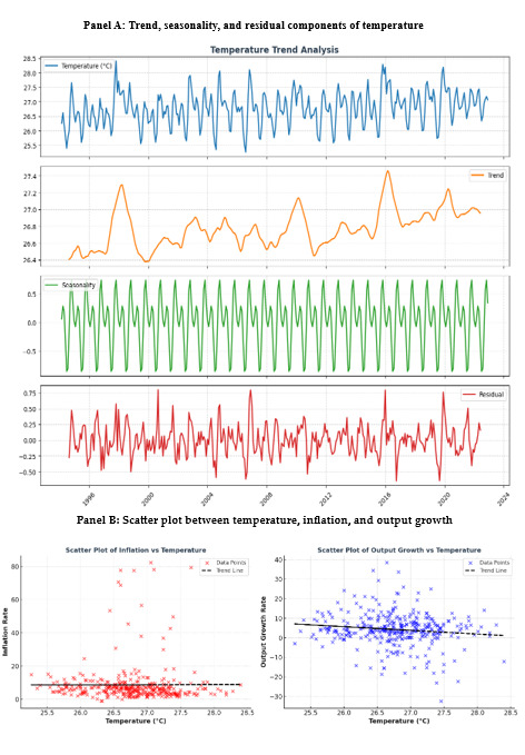
Figure 1 (see Panel A) displays both trends and seasonal patterns in average temperature. The first section highlights notable fluctuations and distinct patterns in the temperature trend. The second sub-plot reveals an upward trajectory, indicating that temperatures have risen over time. The following sub-plot focuses on seasonality, demonstrating clear recurring changes in temperature. The final section presents residuals after removing seasonal components from the data. Since there was clear evidence of seasonality, we incorporated this factor into our temperature estimation model. Figure 1 (see Panel B) displays scatter plots; the first illustrates the link between temperature and inflation, while the second shows how temperature relates to output growth. The graphs indicate that as average temperature rises, inflation tends to increase, demonstrating a positive relationship. Conversely, the second graph reveals a negative correlation between temperature and output growth rate, implying that higher temperatures are associated with reduced output growth.

Figure 1.Temperature dynamics and their relationship with inflation and output growth

Note: Panel A displays average temperature, its trend, seasonality, and the residual in sequence across the subplots. Panel B plots the scatter plot between average temperature and inflation rate, temperature and output growth rate.

Prior to estimating the VAR model, we conducted a unit root test to assess whether the variables were stationary. The scatter plot revealed volatility in both inflation and output. To account for possible structural breaks in the data, we applied the Narayan and Popp (2010) unit root test, with results presented in Table 1. Our analysis showed that temperature, output, and inflation rate were stationary in both M1 and M2 models. In contrast, money supply was non-stationary in the M1 model but stationary in the M2 model. As a result, we transformed the money supply variable by taking its first difference to ensure stationarity before performing the VAR estimation.

Following the unit root test, we evaluated the causal relationship between temperature, inflation, and output growth rate, with the results presented in Table 2. The first null hypothesis, that is temperature does not Granger-cause output, is rejected, indicating that temperature has a statistically significant impact on output growth within the economy. Similarly, the fourth null hypothesis, that is temperature does not Granger-cause inflation, is also rejected, suggesting that temperature Granger-causes inflation. However, the reverse causality hypotheses are not rejected, which implies that neither output nor inflation Granger-cause temperature.

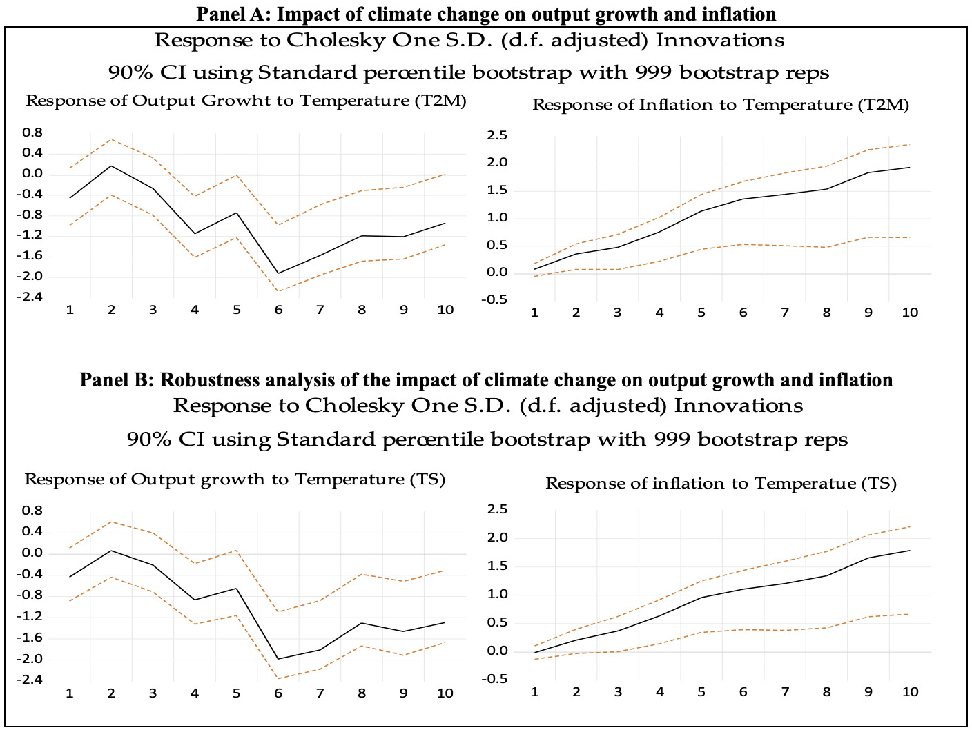
After the Granger causality test, we employed the structural VAR model to further analyze the effects of climate change on inflation and output growth rate. The model demonstrated stability, lacked autocorrelation, and exhibited no heteroscedasticity issues. Variable ordering was determined using Cholesky-dof adjusted decomposition. Figure 2 panel A illustrates the impulse response functions for both output growth rate and inflation rate. The first graph reveals how economic growth responds to a temperature shock, showing that an increase in temperature negatively influences Indonesia’s output growth rate. This effect is primarily transmitted through disruptions to outdoor economic activities, which consequently impact other sectors. These findings are consistent with existing literature, such as Burke et al. (2015), who also reported adverse effects of temperature on economic growth. Additionally, the study observes that the effect of temperature evolves over time; while initially limited, it becomes substantially significant from the fourth month onward, highlighting a lagged impact. This observation aligns with Dell et al. (2012) and Moore and Diaz (2015), who identify a delayed effect of temperature on economic growth.

The right-hand graphs (Panel A of Figure 2) demonstrate the response of inflation to a positive temperature shock, indicating that higher temperatures exert a positive and statistically significant effect on inflation. In practical terms, increases in temperature contribute to rising inflation rates. This phenomenon can be attributed to the influence of elevated temperatures on labour supply, agriculture, and related sectors (IMF, 2023). The findings further reveal that the long-term impact of climate change on inflation intensifies over time, signifying a stronger influence in extended periods.

For the robustness check, we employ an alternative climate change measure, utilizing Earth’s skin temperature (TS) data from NASA, with results presented in Figure 2 (see Panel B). The left panel of the figure depicts the effect of climate change on output growth, while the right-hand graphs demonstrate the relationship between temperature and the economy’s inflation rate. The analysis indicates that this alternative temperature proxy negatively affects output growth and is associated with increased inflation. Therefore, our conclusions remain consistent when adopting this alternative measure of climate change.

Figure 2.Impact of climate change

Note: Model in Panel A includes the temperature (T2M), output growth, inflation and money supply. We control for structural breaks by incorporating the dummy variables for 2000M1 and 2003M11 while model in Panel B includes the temperature (TS), output growth, inflation and money supply. We control the structural break by incorporating the dummies (2000M1 and 2003M11) and global variables proxied by US GDP and policy rate.

IV. Concluding Remarks

This study examines the effects of climate change on inflation and output growth in Indonesia. Monthly data spanning from March 1994 to December 2022 were utilized, with Granger causality and SVAR methodologies employed for analysis. Findings from the Granger Causality test indicate that temperature serves as a causal factor for both inflation and output growth; specifically, rising temperatures are associated with increased inflation rates and diminished economic output. Additionally, SVAR estimation results demonstrate that positive temperature shocks contribute to higher inflation and negatively affect output growth.

From a policy standpoint, these empirical insights underscore that temperature shocks place upward pressure on inflation and constrain output growth within Indonesia. Consequently, macroeconomic and climate policies should not be formulated independently. It is recommended that monetary policy frameworks include climate-sensitive indicators for effective inflation targeting, while fiscal policy should prioritize investments in climate-resilient infrastructure, agriculture, and social protection, particularly in the most vulnerable regions. An integrated approach encompassing monetary, fiscal, and environmental policies is vital to mitigate the adverse impacts of climate shocks on inflation stability and economic growth.