I. Introduction

The objective of this study is to examine the role of disease-based uncertainty in predicting energy stock markets. The motivation for our study is threefold. First, the current COVID-19 pandemic has shown that stock markets and financial markets of many countries are sensitive to the pandemic (see, Bouri et al., 2020). Second, uncertainty that created by pandemics that impact health have significant influence on investors’ actions (Baker et al., 2020) and sentiments (HaiYue et al., 2020). Lastly, uncertainty due to the pandemic might restrain the demand for energy which subsequently leads to fall in stock prices and returns (see Sharma & Sha, 2020; and Sha & Sharma, 2020).

Several studies have documented that the fluctuations in the stock market during the pandemic can be tracked by the uncertainty resulting from economic and non-economic news. For instance, past studies have noted that disasters (Kowalewski & Śpiewanowski, 2020) and epidemics (C. D. Chen et al., 2009; M.-H. Chen et al., 2007; Ichev & Marinč, 2018; Salisu & Adediran, 2020; Salisu & Vo, 2020) significantly influence the stock market. To be more specific, Salisu & Adediran (2020) unveil that uncertainty due to the pandemic tracks well the volatility in energy markets in both in-sample and out-of- sample tests. Furthermore, Salisu & Vo (2020) document that investors started to sell off their stocks during the early stages of the COVID-19 pandemic due to fear of loss. On the other hand, Liu et al. (2020) show that COVID-19 exerts a positive influence on the crude oil and stock returns.

To the best of our knowledge, there is limited understanding about the influence of uncertainty caused by pandemics on the Asia-Pacific energy stocks. On this note, we extend the literature by determining the role of pandemics in predicting energy stocks for the Asia-Pacific market. We partition our estimation into two by considering the full sample of data and the COVID-19 sample of data. To this end, we utilize the novel nonparametric causality-in-quantiles approach recently developed by Balcilar et al. (2018). This approach is capable of testing non-linear causality of the kth order across all quantiles of the entire distribution of stock returns, and is robust to the presence of misspecification errors, structural breaks and frequent outliers, which are commonly found in financial time series data (Balcilar et al., 2018). Another motivation for using the nonparametric quantile-in-causality approach is that when we conduct a test for nonlinearity by applying the Brock et al. (BDS, 1996), the BDS test validates the adoption of the non-linear causality-in-quantiles approach (see for example Fasanya et al., 2021).

The rest of the paper is structured as follows. Section II provides a description of the methodology. Section III discusses the data and results and Section IV concludes.

II. Methodology

This paper follows Balcilar et al. (2018) methodology, which is an extension of Nishiyama et al. (2011) and Jeong et al. (2012) nonlinear causality frameworks. As noted by Jeong et al. (2012), the variable $x_{t}$ (EMV-ID) does not cause $y_{t}$ (energy stock returns) in the $\sigma - quantile$ with respect to the lag-vector of $\{ y_{t - 1},\ldots,y_{t - q},x_{t - 1},x_{t - q}\}$ if

$$\begin{align} Q_{\sigma}\left( y_{t} \middle| y_{t - 1},\ldots,y_{t - q},x_{t - 1},\ldots,x_{t - q} \right)& \\ = Q_{\sigma}\left( y_{t} \middle| y_{t - 1},\ldots,y_{t - q} \right)& \end{align} \tag{1}$$

While $x_{t}$ causes $y_{t}$ in the ${σth}$ quantile with respect to $\{ y_{t - 1},\ldots,y_{t - q},x_{t - 1},x_{t - q}\}$ if

$$\begin{align} Q_{\sigma}\left( y_{t} \middle| y_{t - 1},\ldots,y_{t - q},x_{t - 1},x_{t - q} \right)& \\ \neq Q_{\sigma}\left( y_{t} \middle| y_{t - 1},\ldots,y_{t - q} \right)& \end{align} \tag{2}$$

Thus, they adopt the nonparametric Granger-quantile-causality approach of Nishiyama et al. (2011). To illustrate the causality in higher order moment, they assume:

$$y_{t} = h\left( V_{t - 1} \right) + \vartheta\left( U_{t - 1} \right)\tau_{t}, \tag{3}$$

Where $\tau_{t}$ is the white noise process and $h( \cdot )$ and $\vartheta( \cdot )$ equal the unknown functions that satisfy pertinent conditions for stationarity. Although this specification allows non granger-type causality testing from $U_{t - 1}$ to $y_{t}$, however, it could detect the “predictive power” from $U_{t - 1}$ to $y_{t}^{2}$ when $\vartheta( \cdot )$ is a general nonlinear function. Thus, Equation (3) is re-formulated to account for the null and alternative hypothesis for causality in Equations 4 and 5, respectively.

$$H_{0} = P\left\{ F_{y_{t}^{2}|W_{t - 1}}\left\{ Q_{\sigma}\left( y_{t} \middle| W_{t - 1} \right) \right\} = \sigma \right\} = 1, \tag{4}$$

$$H_{1} = P\left\{ F_{y_{{t}}^{2}|W_{t - 1}}\left\{ Q_{\sigma}\left( y_{t} \middle| W_{t - 1} \right) \right\} = \sigma \right\} < 1, \tag{5}$$

We obtain the feasible test statistic for testing the null hypothesis in Equation (4). With the inclusion of the Jeong et al. (2012) approach, Balcilar et al. (2018) overcome the issue that causality in mean implies causality in variance. Specifically, they interpret the causality in higher-order moments through the use of the following model:

$$y_{t} = h\left( U_{t - 1},V_{t - 1} \right) + \tau_{t}, \tag{6}$$

Thus, the higher order quantile causality is:

$$\begin{align} H_{0} = P\left\{ F_{y_{t}^{k}|W_{t - 1}}\left\{ Q_{\sigma}\left( y_{t} \middle| W_{t - 1} \right) \right\} = \sigma \right\} = 1,& \\ \ for \ k = 1,2,\ldots,k,& \end{align} \tag{7}$$

$$\begin{align} H_{1} = P\left\{ F_{y_{{t}}^{k}|W_{t - 1}}\left\{ Q_{\sigma}\left( y_{t} \middle| W_{t - 1} \right) \right\} = \sigma \right\} < 1,& \\ \ for \ k = 1,2,\ldots,k.& \end{align}\tag{8}$$

Overall, we test that $x_{t}$ Granger causes $y_{t}$ in ${σth}$ quantile up to the k-th moment through the use of Equation (7) to construct the test statistic of the equation of the first moment (null hypothesis) for each k. Failure to reject the null of k=1 does not translate into non-causality in variance, thus, we construct the tests for k=2. Finally, we test for the existence of causality-in-mean and variance.

III. Data and Results

A. Data and Preliminary Analyses

This paper covers energy stock indices (from which stock returns are computed) of 10 Asia-Pacific countries. These countries are Australia, China, Hong Kong, India, Indonesia, Japan, Korea, Singapore, Taiwan, and Thailand. We use daily data from January 1, 2004 to August 31, 2020 based on data availability. The analyses are conducted using both the full sample and the sample covering the COVID-19 pandemic (01/01/2020 to 31/08/2020). Data on the energy stock indices are obtained from the Thomson Reuters DataStream, and the Infectious Disease Equity Market Volatility (EMV-ID), developed by Baker et al. (2020) and is available for download from http://www.policyuncertainty.com.

Table 1 highlights the relevant descriptive properties of the data. The energy stock indices of all countries considered have positive returns on average, except for China, Japan, and Singapore, which carry negative average returns. However, a large difference is observed between the maximum and minimum values across all series, indicating potential high levels of fluctuations. Based on the standard deviation statistic, the Indonesian stock market is the most volatile while the Australian market experiences the least volatility. Concerning the statistical distribution of the return series, the skewness measure suggests that stock returns of Korea and Singapore are positively skewed, which means they have a long right tail while all others exhibit negative skewness. The kurtosis statistics also reveal that all series are largely leptokurtic (highly peaked). The Jarque-Bera statistic confirms non-normality. Furthermore, we explore the random walk properties of all the variables using the Ng-Perron, and Dickey-Fuller GLS tests, and all series appear to be stationary at the 5% significance level. This is a pre-requisite for our causality analysis.

B. Results

We begin the analysis by examining the causal effect of uncertainties due to infectious disease outbreaks on the returns of each of the energy stock indices from a linear perspective.^[1] However, we perceive this may likely be due to nonlinearity in the series, as the presence of heavy tails, excess kurtosis, and non-normality are suggestive of the possibility of the nonlinear nature of the series.

Furthermore, to confirm our suspicion, we conduct a more formal test (BDS test) developed by Broock et al. (1996) to establish the presence of nonlinearity in the series. The BDS test results for the full sample and the COVID-19 regimes are reported in Table 2. Our analysis shows strong evidence of a nonlinear relationship between EMV_ID and all return series as the null hypothesis of serial dependence is rejected at the highest levels of significance for all countries except China, Indonesia, and Taiwan (Panel B). These results imply strong evidence of nonlinearity in the relationship between EMV_ID and energy stock returns. This means that relying on the linear Granger-causality test may lead to spurious conclusions as it could have suffered from misspecification errors.

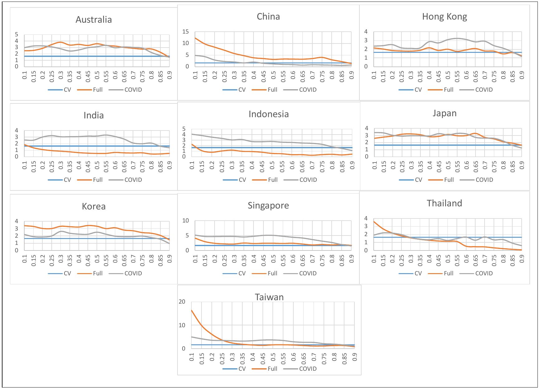
Having established nonlinearity, we turn to the results of the quantiles-based causality tests. Figures 1 and 2 summarize the results of the nonparametric causality-in-quantiles in conditional mean and conditional variance tests, respectively. Each country’s stock-market returns are regressed on the EMV_ID. The horizontal axis shows the quantiles, and the vertical axis shows the test results. The blue horizontal line represents the 90% critical value. The red line represents the results for the full sample, and the grey line represents the results for the COVID-19 sample.

Figure 1:Quantile-based (nonlinear) causality test in conditional mean

Note: The above figures are graphical representations of the causality-in-quantiles in conditional mean and conditional variance results. CV represents critical value at the 10% level.

Figure 2:Quantile-based (nonlinear) causality test in conditional variance

Note: The above figures are graphical representations of the causality-in-quantiles in conditional mean and conditional variance results. CV represents critical value at the 10% level.

Our results show strong evidence supporting the rejection of the null hypothesis of no Granger-causality for both the full sample and for the COVID-19 period. The causal evidence is most significant at the lower and upper quantiles with a few reaching the median region. This indicates a strong causal relationship between uncertainty due to infectious diseases and energy stock returns in the Asia-Pacific region. By implication, investors in the Asia- Pacific energy market may need to consider the likely effects of global pandemics in the valuation of risk-adjusted returns for energy stocks in particular and perhaps in their diversification of financial assets in general. The risk management framework should be reassessed to address new and enhanced risks caused by the COVID-19 pandemic.

IV. Conclusion

In this study, we examine the causal relationship between uncertainties due to infectious disease outbreaks and the Asia-Pacific energy market. We utilize a new dataset by Baker et al. (2020) and employ the nonparametric quantile-based approach. Our findings strongly support the nonlinear causal relationship between uncertainties due to infectious disease outbreaks and the Asia-Pacific energy market. Investors may need to consider the likely effects of global pandemics in the valuation of risk-adjusted returns for energy stocks in particular and perhaps in their diversification of financial assets in general. This conclusion complements the emerging literature on the vulnerability of the energy market to the COVID-19 pandemic.