Tail Risks and Stock Return Predictability: Evidence From Asia-Pacific

I. Introduction

Tail risk gained attention following the 2008/2009 global financial crisis and the recent COVID-19 pandemic, among others. In contrast with banking systems’ financial systemic risk, this concept applies mainly to individual, asset class, and portfolio-level securities (Long et al., 2019). Investors, the direct recipients of the impact of extreme losses, are interested in understanding market dynamics, hence, the desire for empirical evidence on predictors of equity market returns. The predictive capacity of tail risks is currently being examined (Andersen et al., 2020; Chevapatrakul et al., 2019; Long et al., 2019; Salisu, Gupta, & Ogbonna, 2021). Considering tail risks as predictors for returns is premised on its characteristic incorporation of tail thickness information, which circumvents plausible misspecification of distributions or higher-order moments problems (Salisu, Gupta, & Ogbonna, 2021).

Our consideration of the equity markets^[1] of the Asia-Pacific region was motivated by Sharma (2020), who shows that the COVID-19 pandemic heterogeneously affects the country-level volatility of selected Asian economies. We, therefore, extend this study to examine the responses of Asia-Pacific equity markets to an alternative measure of risk—that is, tail risk—following the conditional autoregressive value at risk (CAViaR) specification described by Engle & Manganelli (2004).

In testing the returns-risk hypothesis based on asset pricing theory, the study proceeds with the estimation of (country-specific and US) stocks and oil tail risks by examining the nexus between country-specific stock returns and own tail risk while controlling for global and US stock spillover effects and accounting for salient data features in a distributed lag model (Westerlund & Narayan, 2012, 2015). We show that tail risk has predictive potential for selected major stock indices. We also provide evidence of a significant positive impact of own tail risk on returns. Our model is robust and outperforms the random walk (RW) model. Following the introductory section, Section II focuses on methodology and data description, Section II presents empirical results, and Section IV concludes the paper.

II. Methodology and Data

A. Methodology

The study hinges on the risk-returns hypothesis of the capital asset pricing model (CAPM) that assumes returns respond to market (symmetric) risks (Fama & French, 2004). Stocks and oil tail risks are estimated using CAViaR, which focuses on tail thickness information, rather than the entire distribution (see Engle & Manganelli, 2004) for a detailed technical description). CAViaR reduces the market risks of any portfolio to a single value, and hence, is conceptually simple. The model is:

$$f_{t}(\beta)=\beta_{0}+\sum_{i=1}^{q} \beta_{i} f_{t-i}(\beta)+\sum_{j=1}^{r} \beta_{j} l\left(x_{t-j}\right)\tag{1}$$

where $f_{t}(\beta) \equiv f_{t}\left(x_{t-j}, \beta_{\theta}\right)$ is the $t^{th}$ time $\theta$-quantile of the distribution of portfolio returns formed at $t-1$ ; for notational convenience, subscript $\theta$ in (1) is suppressed. $p=q+r+1$ is the dimension of $\beta$; $l$ is a function of lagged observations; $\beta_{i}f_{t-i}(\beta)$ are autoregressive terms, with $i=1,...,q$ , that ensure smooth quantile changes; $l(x_{t-j})$ links $f_{t}(\beta)$ to observable variables in the information set. The tail risks - adaptive, symmetric absolute value, asymmetric slope, and indirect generalized autoregressive conditional heteroskedasticity (GARCH) are defined as:

$$\begin{align}f_{t}\left(\beta_{1}\right)=&f_{t-1}\left(\beta_{1}\right)+\\ &\beta_{1}\left\{\left[1+\exp \left(G\left[y_{t-1}-f_{t-1}\left(\beta_{1}\right)\right]\right)\right]^{-1}-\theta\right\}\end{align}\tag{2}$$

$$f_{t}(\beta)=\beta_{1}+\beta_{2} f_{t-1}(\beta)+\beta_{3}\left|y_{t-1}\right|\tag{3}$$

$$f_{t}(\beta)=\beta_{1}+\beta_{2} f_{t-1}(\beta)+\beta_{3}\left(y_{t-1}\right)^{+}+\beta_{4}\left(y_{t-1}\right)^{-}\tag{4}$$

$$f_{t}(\beta)=\left(\beta_{1}+\beta_{2} f_{t-1}^{2}(\beta)+\beta_{3} y_{t-1}^{2}\right)^{1 / 2}\tag{5}$$

where equations 2 – 5 are respectively Adaptive, SAV, Asymmetric Slope and Indirect GARCH(1,1) models; $G$ is a positive finite number that makes the model a smoothed version of a step function; $\beta_{1}\left\{\left[1+\exp \left(G\left[y_{t-1}-f_{t-1}\left(\beta_{1}\right)\right]\right)\right]^{-1}-\theta\right\}$ in (2) converges almost certainly to $\beta_{1}\left[I\left(y_{t-1} \leq f_{t-1}\left(\beta_{1}\right)\right)-\theta\right]$ if $G \rightarrow \infty$, with $I$(.) representing the indicator function. While (3) and (5) are symmetric and (4) is asymmetric, equations (3)–(5) are mean-reverting and (2) has a unit coefficient. We generate 1% and 5% VaRs for the CAViaR variants and ascertain “best fit” using the dynamic quantile (DQ) test and % hits.^[2]

Following WN, a distributed lag model for returns that incorporates own, oil, and US-stocks tail risks and accounts for conditional heteroscedasticity, endogeneity/persistence, and day-of-the-week effect (Salisu & Vo, 2020; Yaya & Ogbonna, 2019) is specified. This is to ascertain the impact of own tail risk while controlling for global oil and US stocks spillover effects. The model is defined as:

$$\begin{align}r_{t}=&\ \omega+\sum_{i=1}^{p} \varphi_{i} t r_{t-i}^{c s}+\sum_{k=2 ; \atop i=6,7}^{R} \varphi_{i} t r_{t-1}^{k}\\ &+ \sum_{k=1}^{R} \alpha_{k} \Delta t r_{t}^{k}+\varepsilon_{t}\end{align}\tag{6}$$

where $r_{t}=\ln(P_{t})-\ln(P_{t-1})$ is returns at time $t$; $P_{t}$ is stock price; $\omega$ is the intercept; $t r^{k}=\left(t r^{c s}, t r^{o}, t r^{, u s}\right)$ with $k=1, \ldots, R ; R=3 ; t r^{c s}, t r^{o} \& t r^{u s}$; are country-specific, oil, and US-stock tail risks, respectively; $\varepsilon_{t}$ is a zero-mean idiosyncratic error term. $\alpha_{k} \Delta t r_{t}^{k}$ and $\phi_{i} t r_{t-1}^{k}$ are incorporated to resolve persistence and endogeneity bias. For heteroscedasticity, the model is pre-weighted with the inverted standard deviation of GARCH-type model residuals. The least squares estimation of the resulting equation yields feasible quasi-generalized least squares estimates. We evaluate in-sample predictability (full sample) and out-of-sample forecast evaluation (75% sample) using the Clark and West [CW] (2007) statistic, under forecast horizons $h=$ 5, 10 & 20, and for 1% and 5% VaR.

B. Data

Figure 1.Co-movement in Returns and Tail Risks

This figure shows the co-movement in returns and tail risk. The sample period is from 13th February 2015 to 5th March 2021.

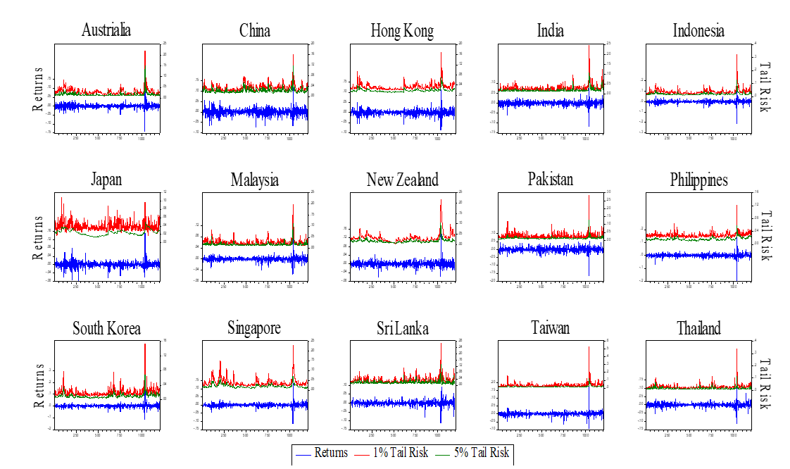
The summarized data (Table 1) comprise daily stock returns of Dow Jones (Australia, Hong Kong, Indonesia, Japan, Malaysia, Philippines, Singapore, South Korea, and Taiwan), Morgan Stanley Capital International (China, India, New Zealand, Pakistan, Sri Lanka, and Thailand), S&P500, and west Texas intermediate (WTI) oil price. The data span 13th February 2015 to 5th March 2021 and are sourced from www.investing.com and the Federal Reserve Bank of St. Louis database for oil data; see https://www.stlouisfed.org/. The optimal (asymmetric and indirect GARCH) models were used to generate the tail risks. All the returns are leptokurtic (heavy tailed), with mixed skewness, suggesting non-normality. Returns and tail risks exhibit ARCH effects and serial correlation while tail risks exhibit persistence, and, hence, our choice of predictors and methodology. Tail risks co-moved with returns (Figure 1).

Table 1.Data summary statistics

This table shows the summary statistics. The rows labelled ‘Out-of-sample’ contain %Hits [DQ] with significance based on closeness of %Hits to stated VaR_percent and statistically non-significant DQ; superscripts “a” and “b” indicate asymmetric slope and indirect GARCH, respectively, as optimal; 1,085 and 120 observations were used for in-sample and out-of-sample tests, respectively. Statistical significance at 1%, 5% and 10% is indicated by ***, ** and *, respectively.

III. Empirical Results

The in-sample parameter estimates of our model for 1% and 5% own tail risks (left panel in Table 2) seem to exhibit mixed trends of statistically significant negative and positive relationships between stock returns and country-specific tail risks, with more cases for the latter. Positive nexuses between returns and own tail risks are found in the cases of Australia, China, Hong Kong, India, Indonesia, New Zealand, Singapore, and Thailand. The positive relationship aligns with Chevapatrakul et al. (2019) and Andersen et al. (2020), implying that tail risks induce a near-term rise (completely disappear) in returns for negative (positive) returns. We find a significantly negative impact of 1% and 5% VaR tail risks of the equity market returns of Japan, Philippines, South Korea, and Sri Lanka. The negative relationship indicates the lack of predictive potential of model predictors for a negative effect of country-specific tail risks, which is an anomaly compared to the literature (Long et al., 2018, 2019). Generally, own tail risks positively impact Asia-Pacific equity market returns, and the results are robust to the tail risks. While incorporating the data period covering the recent COVID-19 pandemic, our study also incorporates optimally determined tail risks (Engle & Manganelli, 2004) with salient data features to ascertain the nexus of returns and tail risk, having controlled for global and foreign stock spillover effects. Hence, we provide more recent and confirmatory evidence of the predictive potentials of own tail risks for returns in Asia-Pacific equity markets.

We also evaluate the out-of-sample forecast performance of our predictive model in comparison with the RW model using CW statistics at horizons $h=$ 5, 10 & 20 to ensure robustness. Our model outperforms the RW model and transcends forecast horizons, countries (except for Thailand at $h=$ 5, 10 & 20 under 5% VaR), and tail risks (right panel in Table 2) and is robust. Tail risks are therefore important predictors for Asia-Pacific equity market returns. This aligns with the established returns–tail risk nexus (Andersen et al., 2020; Chevapatrakul et al., 2019; Long et al., 2019; Salisu, Gupta, & Ogbonna, 2021). In summary, incorporating own tail risks while simultaneously controlling for global and foreign stocks spillover effects and accounting for salient data features improves upon the RW model, which does not account for external data information.

IV. Conclusion

We investigate the predictability of major stocks of the Asia-Pacific region using tail risks and capturing tail thickness information. The tail risks are estimated using four CAViaR model variants: adaptive, symmetric absolute value, asymmetric slope, and indirect GARCH. We find asymmetric slope and indirect GARCH models to be optimal and generate corresponding 1% and 5% tail risks for each country. Our model, which incorporates salient data features, is used to examine the nexus between returns and tail risk while controlling for global oil and US stocks spillover effects. We find country-specific risks to mostly have a positive impact on returns. Tail risks induce a near-term rise in returns on “bad” days (negative returns) and completely disappear on “good” days (positive returns). Our results are robust.