Estimation of Life Insurance Asset Value From Household Survey

I. Introduction

Life insurance is mainly targeted to insure against the mortality risk of the insured. The role of life insurance in typical household assets is often ignored. Life insurance usually carries some accumulated cash value which is essentially a form of household savings. For example, if an insured household elects to discontinue their life insurance policy, they would usually receive a discounted amount of premiums called “surrender value” from the insurer. Using the Survey of Consumer Finances, Bricker et al. (2017) show that 19.0 percent of U.S. households held life insurance assets in 2019; the average cash value was $41,000, which accounted for nearly 5 percent of total household assets.^[1] However, a life insurance policy can be worth more than the surrender value in the secondary market. The pricing of life insurance policies is ambiguous in real scenarios, and the asset value of life insurance policies is also often overlooked or outright ignored in many economic studies concerning calculating household assets or wealth for various reasons.^[2] Such omissions result in household asset values being underestimated and as such bias the measures of wealth inequality. Therefore, a scientific method is required in place to compute the asset value of life insurance with limited information of households.

In this study, we propose a maneuverable method, which combines a multi-disciplined knowledge of demography and actuarial science, to estimate the asset value of household life insurance using limited information from a typical household survey. According to the division of discipline and techniques, this paper can be naturally divided into two parts. First, we obtain historical life tables and apply the Lee-Carter model to pin down a group of parameters as well as to project individuals’ future mortality risk across age and time. Second, we make use of the individual’s characteristics, the basic information of the life insurance policy, and forecasted mortality risk to estimate the asset value of a life insurance policy to compute both individual and household life insurance asset value by employing the concept of net level premium reserve (NLPR) in actuarial science (Gerber, 1990; Møller & Steffensen, 2007).

The rest of the paper is organized as follows. In section II, we introduce our methods of forecasting individual mortality risks and calculation of life insurance asset value. In section III, we use individual demographic and life insurance information from the 2013 China Household Finance Survey (CHFS) as an application, illustrate the impact of life insurance assets on wealth inequality, and discuss our findings with some stimulating facts on life insurance holding in China. We then present our conclusions in Section IV.

II. Methodology

A. Estimation and Forecasting of Individual Mortality Risks

We employ the mortality forecasting model by Lee & Carter (1992). Let m(x,t) to be the matrix of central death rates for age $x$ in year $t,x=1,2,\ldots,N, t=1,2,\ldots,T$. Then the matrix of death rates can be modeled by

$$ln[\mathbf{m}(x,t)]=\mathbf{a}_x+\mathbf{b}_x\mathbf{k}_t+\varepsilon_{x,t}\tag{1}$$

or

$$\mathbf{m}(x,t)=e^{\mathbf{a}_x+\mathbf{k}_t\mathbf{b}_x+\varepsilon_{x,t}}\tag{2},$$

for age-specific constants $\{\mathbf{a}_{x}\}$ and $\{\mathbf{b}_{x}\}$ and the time-varying index $\{\mathbf{k}_{t}\}$. Since the model is undetermined, as noted by Lee & Carter (1992), we can further impose restrictions such that the $\mathbf{b}$'s are normalized to sum to one and the $\mathbf{k}$'s sum to zero. Therefore, $\mathbf{a}_{x}$ can be interpreted as an average age-profile; $\mathbf{k}_{t}$ indexes the intensity of mortality over time and declines almost at a constant rate with stable variability; $\mathbf{b}_{x}$ illustrates how sensitive the mortality rates decline for a specific age group in response to the changes in $\mathbf{k}_{t}$. The error term, $\mathbf{\varepsilon}_{x,t}$, is assumed to have zero mean and variance $\mathbf{\sigma}_{\varepsilon}^{2}$, reflects some particular age-specific historical influences not captured by the model. We use the singular value decomposition (SVD) method (Good, 1969) to obtain the parameters of $\{\mathbf{a}_{x}\}$,$\{\mathbf{b}_{x}\}$, and $\{\mathbf{k}_{t}\}$.

Having reduced the time dimension of mortality to a single index $\mathbf{k}_{t}$, Lee & Carter (1992) use statistical time series methods to model and forecast this index. Assume $\mathbf{b}_{x}$ remains constant over time and forecast future values of $\mathbf{k}_{t}$ with a standard univariate time-series model. In their application to U.S. mortality they discovered that the index behaves like a simple random walk with a drift,

$$\mathbf{k}_t=\mathbf{k}_{t-1}+d+e_t,t=1,2\ldots,T,\tag{3}$$

where $d$ is the drift, and $e_{t}$ are independent error terms with mean zero and variance $v$.^[3]

The maximum likelihood estimate of the drift parameter is $\hat{d} = \frac{{\hat{\mathbf{k}}_\text{T}-\hat{\mathbf{k}}_1}}{t-1}$. Following Girosi & King (2008), we can estimate the future values of $\mathbf{k}_{t}$ by assuming the same ARIMA(1,0,1) behavior,

$$\mathbf{\hat{k}}_t=\mathbf{\hat{k}}_{1}+(t-t_1)\hat{d}.\tag{4}$$

Also, the variance of $\mathbf{k}_{t}$ increases with the forecast horizon $t$. Using the law of iterated expectations, it is not difficult to showcase that starting from a fixed value at time $t_{1}$, the variance of $\mathbf{k}_{t}$ is $var(K_t)=(t-t_1)v$.

B. Computation of Individual’s Net Level Premium Reserve

We estimate the asset value of life insurance policies by introducing the concept of net level premium reserve (NLPR), which is the balance between the expected present value of amounts to be paid into and out of the insurer under the policy (Gerber, 1990). We have retrospective and prospective methods to compute NLPR (Mikola, 2007; Slud, 2006). Both methods will produce the same level of reserves at the end of any given year under the same actuarial assumptions.

B.1. The retrospective reserve

The retrospective reserve represents the net premiums collected by the insurer for a particular block of policies, plus interest earned at an assumed rate, less the amount paid out as death claims.

$$V_{\alpha,t}=\sum_{s=t_0}^t(C_s-B_s)(1+r)^{t-s}\tag{5}$$

where $C_{s}$ and $B_{s}$ are premiums and dividends incurred at year $s$, and $r$ is the interest rate assumed as a constant in the past.

B.2. The prospective reserve

The prospective reserve is derived in the light of dynamic programming with a finite terminal date in macroeconomics. The prospective reserve is the difference between the present value of future benefits and the present value of future net premiums. It assumes that at the end of the terminal age, $\Omega$, an individual will die at probability 1 and the death benefit would be acquired. Therefore, the cash value for the terminal year, $V_{\Omega}$, is the discounted value of death benefit, $\Phi$, minus the cost of the insurance contract renewal, i.e., premium $C_{\Omega}$, if any:

$$V_\Omega=-C_\Omega+\frac{\Phi}{1+r}.\tag{7}$$

While for every other age α, the cash value $V_{\alpha,t}$ for the specific time t is the difference between expected benefits and cost of the contract renewals. Here, the expected benefit is the probability of dying for the specific age and time, $q_{\alpha,t}$, times the discounted death benefits plus the product of the probability of survival, ${1 - q}_{\alpha,t}$, and discounted cash value for the following year:

$$V_{\alpha,t}=-C_\Omega+q_{\alpha,t}\frac{\Phi}{1+r}+(1-q_{\alpha,t})\frac{V_{\alpha+1,t+1}}{1+r}.\tag{8}$$

Equation (7) and (8) form a recursive structure of the asset value of a life insurance.

III. Application and results discussion

In this section, we apply the aforementioned method by employing historical life tables and the 2013 China Household Finance Survey.^[4]

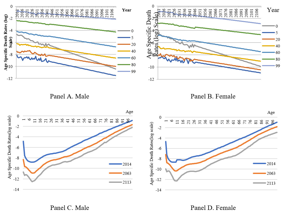
The first stage mortality risk forecasting requires long-term historical life tables for the identification of parameters in the Lee-Carter model. Since the historical life tables of the Chinese population is limited and updated irregularly, we use the annual life table of Hong Kong 1971-2016 as a substitute due to its geographic and ethnic similarities with mainland China.^[5][6] Some selected age-specific mortality rates are plotted in Figure 1 (Panel A and Panel B) and mortality rates over the life cycle in some selected years are plotted in Figure 1 (Panel C and Panel D).

Figure 1.Age-specific death rates

Notes: The panel A and B show the projected male and female mortality rates (in log scale) over time for some selected age groups. The panel C and D show the male and female mortality rates (in log scale) over the life cycle in some selected years.

After obtaining the matrix of forecasted mortality rates, we then match the age and gender-specific mortality risks with the demographic characteristics of the insured individual in household surveys. For illustration purposes, we use the 2013 China Household Finance Survey (CHFS) which provides some fundamental information about life insurance policies like insured amount (i.e., death benefits), dividend, premium, premium payment frequency and terms, etc. By applying the methods from Section II. B, we can calculate the net level premium reserves (NLPR) of individual life insurance policies. It is worth noting that the retrospective reserve of equation (6) is increasing at a compounding interest rate, while the prospective reserve in equation (8) is decreasing in the discounting interest rate. As shown in Figure 2, the averages of individual retrospective and prospective reserve values in the 2013 CHFS sample intersect at an interest rate of approximately 2.5%, which is very close to general interest rates in China in 2013. Given the principle that both methods will produce the same level of reserves if all other conditions are equal, we can pin down the interest rate at the mentioned level for further computations.^[7]

Figure 2.Average retrospective and prospective reserves.

Notes: Using 2013 China Household Finance Survey (CHFS) data, this figure shows the computed individual average net level premium reserve (NLPR) as functions of interest rate by prospective and retrospective methods, respectively. The two functional values intersect at interest rate around 2.5%, which is very close to general interest rates in China in the same year.

We can then aggregate the NLPR of individual members to the household level. The summary statistics of prospective reserves with various discount rates are reported in Table 1.^[8]

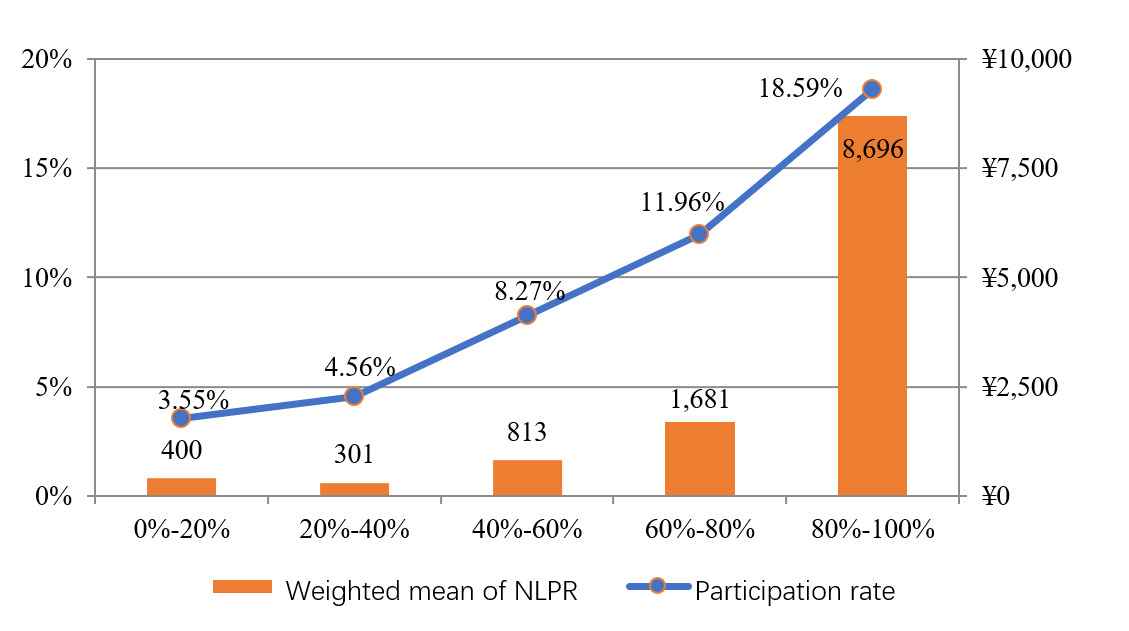
If we consider the results as a benchmark when the discount rate is set at 2.5%, several findings concerning household life insurance behavior in China or other countries in general deserve to be highlighted and discussed. First, current life insurance participation in China is considerably low compared with developed economies such as the United States (see Bhutta et al., 2020). According to our calculation, only 1,378 of 28,141 households in the sample hold a positive life insurance asset, which only accounts for about 4.90% of the total. Second, the life insurance asset value is non-negligible. For the life insurance holders, the life insurance asset value is 52,904 yuan or equivalently 7.62% of the average household wealth within the sample group. This share is much smaller, 0.35%, among all households due to low participation. Given the high potential of commercial life insurance penetration in developing countries like China, it is essential to include the life insurance asset component as soon as possible to prevent future biases of household wealth calculation. Third, the fact that the inclusion of life insurance assets value results in a widening of wealth inequality implies that life insurance is disproportionally held by wealthy households. This conjecture can be confirmed by Figure 3, which shows life insurance participation and average NLPR are increasing on wealth quintiles.^[9] Thus the omission of life insurance assets also underestimates wealth inequality.

Figure 3.Life insurance participation rates and average NLPR along the wealth distribution

Notes: This figure shows the life insurance participation rate (left scale) and weighted mean of NLPR (right scale) for different wealth quintiles. Amounts are in 2013 RMB and are weighted by household sampling weights.

IV. Conclusion

The omission of household life insurance assets underestimates household asset value and biases the measurement of wealth inequality. The surrender value of life insurance is not a good substitute because: 1) it usually has a lower evaluation than a policy’s market value, and 2) households may not have full information on this time-variant value. Thereby, we propose a method to estimate the cash value of household life insurance assets by combining the mortality risk forecasting models in demographics and the concept of the net level premium reserve (NLPR) in actuarial science. Such a method can be easily applied to household survey data with basic information on individual characteristics and life insurance policy. Given the increasing importance of life insurance in household financial portfolios, it is essential to incorporate this method into the calculations of household wealth at the earliest possible time.

Acknowledgment

The authors are grateful to reviewers and editors of the journal for helpful comments and suggestions. The authors would also like to thank Teng Li, Xiaoquan Wang, Randong Yuan, Shenghao Zhu and participants of the 2018 Chinese Economist Society (CES) Annual China Conference for their helpful suggestions and comments. All remaining errors are ours. This work is supported by the Fundamental Research Funds for the Central Universities (project number JBK1801004) and National Natural Science Foundation of China (project number 71903156).