Partisan Conflict and Government Spending: New Evidence From the United States

I. Introduction

The government tends to switch economic policies to increase their votes in elections (Bove et al., 2017; Philips, 2016). Incumbents commonly increase public expenditures and raise aggregate government spending. Electoral incentives can induce budget shifting, leading to more observable consumption than investment in public goods (Bove et al., 2017; Drazen & Eslava, 2010). Therefore, to demonstrate their proficiency, incumbents prefer to shift the composition rather than the level of government spending. The shifting of government expenditures can decrease the budget in a sector while increasing government spending in another. Earlier analyses of the political impact on budget shifting are focused on the political budget cycles that arise during elections (e.g. Bove et al., 2017; De Haan & Klomp, 2013; Klomp & De Haan, 2012; Philips, 2016). Klomp and de Haan (2012) and De Haan and Klomp (2013) emphasize that partisan conflict (PC) discourages aggregate government spending.

In this paper, we investigate the potential link between PC and government spending in the United States. Specifically, we employ a new political variable measurement, the PC index developed by Azzimonti (2014, 2018), to analyze the impact of government spending on political risk shock. Our results show that higher PC tends to reduce government expenditures. Specifically, the US budget in the education sector and regarding income security in the welfare sector is the most significantly negatively affected by an increase of PC shock.

This paper makes two contributions to the literature (Azzimonti, 2019; Cheng et al., 2016; Gupta et al., 2019; Hankins et al., 2016; Hoke, 2019; Jia et al., 2020). The first is that we quantitatively investigate how the behaviors of political parties affect fiscal policy dynamics by employing the PC index. The second is that this paper extends the literature on how exogenous shocks affect disaggregated government spending the short term.

II. Data and Methodology

A. Data

The PC index is constructed based on the textual analysis of newspaper articles. In particular, PC is computed based on a semantic search approach to measuring newspaper coverage as the frequency of articles reporting political disagreement about government policy—both within and between national parties—normalized by the total number of news articles within a given period. We use aggregate annual PC index data for the United States from 1981 to 2018, extracted from the Federal Reserve Bank of Philadelphia based on data availability. To investigate the response of macroeconomic variables to PC, we use other variables, including output, taxes, and aggregate government spending. We assess the ways in which PC has a stronger effect on disaggregated US government spending, including defense, economic affairs, income security, disability, welfare and social services, education, health, general public services, recreation, and culture.

Figure 1 shows nine categories of government expenditure that have grown steadily from 1981 to 2018. We can see that almost all election years show an uptrend in the PC index (Azzimonti, 2014). This implies that rumors of political disagreement around political agendas are more frequent than during non-election periods, especially after a new president has been elected. The responses of nine government spending sectors vary but are consistent with the increase in PC around election years. PC peaked by more than five points during the 2012 election before it decreased around 2013–2014 due to the calmness of the post-election period. The pattern of government expenditure in income security for disability and the housing and community service sectors increases as PC increases, whereas other sectors show downtrend patterns.

Figure 1.Time trend of PC and government expenditure in different sectors

The right axis corresponds to the partisan conflict.

B. Econometric model

To explore how PC affects federal government spending, we build a vector autoregressive (VAR) model of nine different expenditures, including national defense, economic affairs, income security in disability, income security in welfare and social services, education, health, general public services, housing and community services, and public order and safety.

We employ impulse response functions to the shock in the PC index variables for government spending, taxes, and output in the aggregate and the nine sectors of the US government spending sequentially. We also use variance and historical decomposition to predict the impact of the PC shock for each sector. Variance decomposition is used to analyze each variable’s contribution to the multi-step forecast error variance of other variables. We use the fourth, 12th, and 20th time of horizon to predict the forecast error variance decomposition of nine sectors of US government expenditures under a US PC index shock. To explore historical fluctuation in the VAR model, we also apply historical decomposition to each US government spending sector.

We consider a structural VAR model following the strategy of Auerbach and Gorodnichenko (2012) and obtain orthogonal shocks by using a Cholesky decomposition, as follows:

$$X_{t}=\sum_{i=1 \cdots p} A_{t} X_{t-i}+u_{t}\tag{1}$$

where $X_{t} = \left\lfloor {PC}_{t}\ G_{t}\ T_{t}\ Y_{t} \right\rfloor.$ Here, ${PC}_{t}\text{PC}_{t}$ is the level of US PC, $G_{t}\ \text{G}_{t}$ is total federal government spending, $T_{t}\ \text{T}_{t}$is tax revenue, and $Y_{t}\ \text{Y}_{t}$is the gross domestic product (GDP). This kind of Cholesky order implies that PC, as an exogenous driver, has contemporaneous effects on other variables in the United States. We proceed sequentially with our analysis using a similar strategy as in equation (1) by replacing the government spending variable, $G_{t}G_{t}$, with each of the nine sectors of US government expenditures. We estimate the sequential model in line with the work of Fernández et al. (2017). The VAR is stable, so that impulse response functions can be constructed.

III. Results and Discussion

A. Impulse response function

The literature on the impact of PC on fiscal policy mainly focuses on fiscal surplus and deficit (Gupta et al., 2019). In Figure 2, it is straightforward to see that PC has a negative impact on government purchases, taxes, and the GDP. Total government purchases decline due to increasing PC, with the lowest value of around -0.3 percent in the fourth month. Katsimi and Sarantides (2012) find the electoral cycle to have a negative effect on direct taxes. Similarly, our results confirm that political parties’ lower taxes in the face of higher PC in a tight political period. Of the three macroeconomic variables, government purchases exhibit the greatest delay in response. In addition, we conclude that the impact of PC on output is statistically significant. The GDP decreases the least in response to an increase in PC over the sample period. The negative response of output occurs two months after the lowest peak impact of about 0.2 percent. Our result differs from that of Hoke (2019), who finds PC to have no impact on output.

Figure 2.Impulse response function

The shaded areas correspond to 68 percent error band intervals.

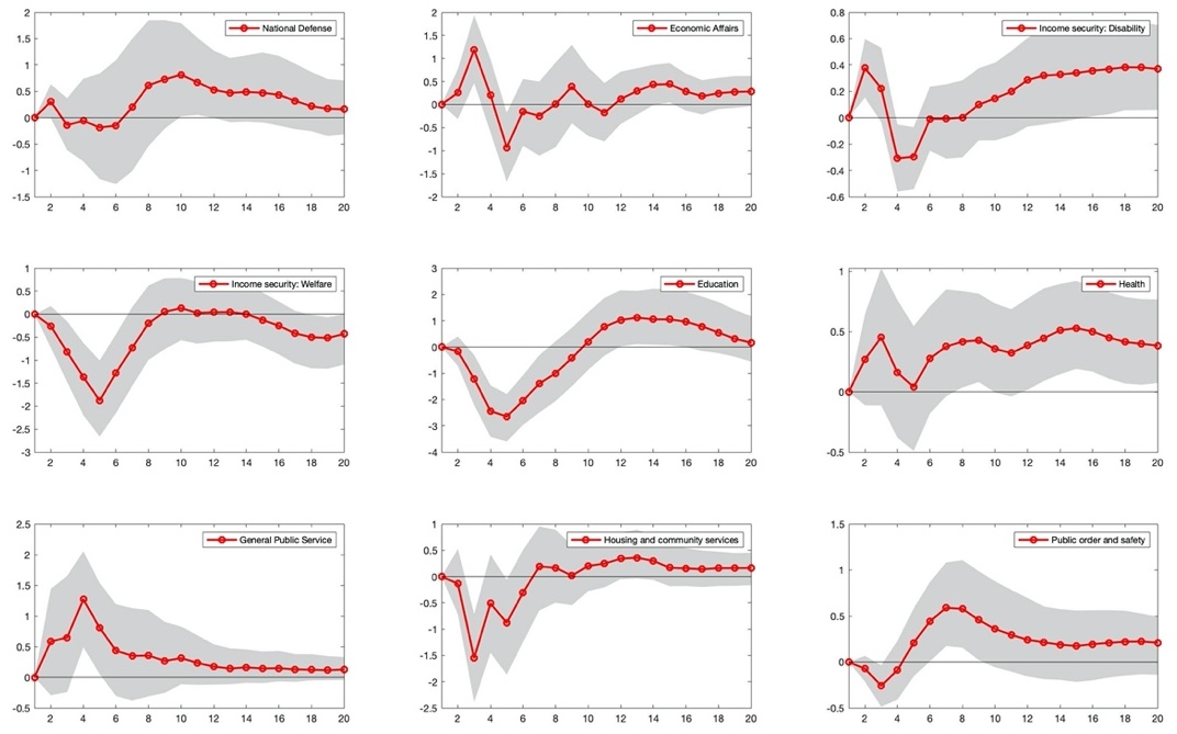
Figure 3 reveals the effects of PC on disaggregated government spending. In the short run, national defense has a positive response to an increase in the PC. However, income security for welfare responds negatively to PC, with the lowest peak below 1.5 points in the fifth year, which then reverses until the 10th year. These findings confirm the study of Bove et al. (2017), in which politicians face a trade-off between butter and guns, implying that policymakers improve or leave the social welfare budget as a constant or decrease military budgeting expenses. In addition, the positive response of economic affairs to PC means that incumbents increase the budget enormously to improve international activity, such as export and other international agreements. It is worth pointing out that the education sector has the most negative response in terms of disaggregated US government spending to PC in the fifth year. Our empirical results are consistent with the literature. For instance, Galli and Rossi (2002) show that electoral cycles tend to decrease the government budget in Germany’s education sector.

B. Variance decomposition

To understand the contribution of the PC shock in the empirical model, we perform a variance decomposition of the variables contained in the VAR system at different horizons. Table 1 shows the results of variance decomposition for disaggregated government spending. At the horizon of the 20th period, we find that US PC has a nontrivial effect on government expenditures in all sectors. US PC explains more than one-quarter of the movement in national defense. In addition, US PC accounts for more than 15% of the fluctuations in economic affairs, social welfare, and housing and community services.

C. Historical decomposition

Historical decomposition allows us to calculate the deviation of the variables of interest from their unconditional means, driven by different types of structural shocks in each period. Figure 4 presents the historical decomposition of disaggregated government spending from 1985 to 2018. Overall, PC contributes strongly to fluctuations in national defense, in comparison to the other sectors, significantly increasing it from 1990 to 1999, from 2000 to 2008, and from 2014 to 2018. The change in education is also of interest. We find that PC contributes to the most significant negative change in the budget in the education sector, with the largest change of -0.2 in 1999 and 2000 and peaking above 0.3 percent in 2010. We find that the budget in the education sector decreases in the initial period due to PC shock, rather than to taxes and output shocks. However, after 2003, output and taxes jointly contributed to the increase of government spending in the education sector.

Figure 3.Impulse response function based on the VAR sequential estimation

The shaded areas correspond to 68 percent error band intervals.

Figure 4.Historical decomposition

The unit is in percentage.

IV. Concluding Remarks

We employ the PC index constructed by Azzimonti (2014) in the United States to identify the responses of aggregate and disaggregated government spending to a PC shock by estimating a VAR model. First, the results of the impulse response function show that aggregate government spending responds negatively to PC shock. Most of the disaggregated government spending measures have a similar response as aggregate spending, except for the health and general public service sectors. Second, the national defense, economic affairs, and housing and community service sectors present high levels of variance decomposition due to PC shock. Third, the results of historical decomposition are consistent with the results of the variance decomposition. PC contributes to the peak in overall expenditures, especially government spending in the education sector. Therefore, lowering PC can help avoid disagreements about fiscal expenditures in education, social welfare, and other areas, as well as improve the overall level of social welfare.

Disclosure Statement

No potential conflict of interest was declared by the authors.

Funding Information

The National Social Science Fund of China (20BTJ015)