Expectations Channel of the Monetary Policy in India: A Structural Factor Augmented VAR Approach

I. Introduction

The primary goals of monetary policy in central banks are price stability and output growth. Price stability becomes more important in the process of sustainable long-term output growth. The Reserve Bank of India Act 1934 mandates 4 percent inflation target with +/- 2 percent band flexibility. To achieve inflation targets, anchoring inflationary expectations assume prime importance for a central bank. Woodford (2003) and Boivin (2011) emphasized the importance of the management of expectations by monetary policy. Credible forecasts can act as a focal point for macroeconomic expectations especially in emerging markets where information tends to be scanty (see Goyal & Parab, 2021).

It is well known that expectations are not directly observed and inference about their formation is derived from models that assume a specific process of expectations formation. In India, data for future inflation expectation forecasts are available in the quarterly inflation expectations survey data of households (IESH) and the professional forecasters’ inflation forecasts collected by the Reserve Bank of India (RBI).

Coibion and Gorodnichenko (2015) raise questions about the process of expectations formation, and how creating the best empirical model for these expectations formations remain an unsolved mystery. Shaw (2019) also proved that quarterly inflation expectations survey data of households (IESH) do not form results based on the rational expectations principle.

Generally, students of economics are taught to believe that what people actually do and not what they say. Hence, subjective statements make one sceptical about measuring inflation expectations, thus attracting a lot of criticism. Given the historical data on actual inflation, we calculated data on “actual future inflation” as a proxy for inflation expectations (see Minella & Souza-Sobrinho, 2013).

This paper analyses the linkages between macroeconomic variables and the expectation variable in a ‘data-rich environment’. Several studies (Friedman & Schwartz, 1963; Sharma & Nurudeen, 2020) have been conducted that analyse the relationship between these variables. However, the expectations channel is not studied due to its complex nature, hence, this study’s attempt to fill this very significant research gap.

Besides, our approach is one of the first few FAVAR approaches implemented in the Indian context. This is an approach which is structural and provides an economic interpretation of the results. Also, this paper is one of the first to analyse the performance of expectations channels of monetary policy transmission in India.

The rest of the paper is structured as follows. Section II discusses the data sources and methodology in detail. Section III explains the results of the empirical analyses. Section IV concludes the paper.

II. Data and Methodology

The study examines 52 variables^[1] divided into 4 factors, namely: interest factor, the money supply factor, the inflation factor, and the output factor. These factors, along with the “actual future inflation” data, are studied in a Structural Factor Augmented VAR framework. The factors were extracted using Principal Component Analysis (PCA)^[2] and selected on the basis of the variables that are best explained by it. The variables in each factor are close alternatives of each other.

Introduced by Bernanke, Boivin and Eliasz (2005), this modelling approach presents observable and unobservable series. The observables are those series which can be directly measured. Correspondingly, non-observables are those series which cannot be directly measured, for example, output gap. Since output gap cannot be observed, factors extracted can be used to represent the series. In either case, both observables and non-observables are allowed to follow a VAR process. Belviso and Milani (2006) also mention the PCA factor extraction method and further a Structural FAVAR analysis (SFAVAR).

To understand the application of SFAVAR methodology, firstly, we demonstrate the factor extraction process. Thus, consider the equation below in which $X_{t}$ is a vector with large macroeconomic variables. Now, to disentangle $X_{t}$ from observed and unobserved elements reported by $Y_{t}$ and $F_{t}$ respectively, we have the following relation:

$$X_{t} = \tau_{i}*F_{t} + \tau_{j}*Y_{t} + \varepsilon_{t}\tag{1}$$

where $X_{t}$ is a $N*1$ vector of macroeconomic variables, $\tau_{i}$ and $\tau_{j}$ are vectors of $N*M$ factor loadings and structural coefficients, respectively. The indicator $\epsilon_{t}$ is the random disturbance term with zero mean and constant volatility. Equation (1) could be augmented in VAR framework and could be re-written as follows:

$$\begin{bmatrix} F_{t} \\ Y_{t} \\ \end{bmatrix} = Q1 + Q2(L)\begin{bmatrix} F_{t} \\ Y_{t} \\ \end{bmatrix} + \ v_{t}\tag{2}$$

where $Q1$ is the vector of intercepts, $Q2$ is the matrix of factor loadings and $\upsilon_{t}$ is the $K*1$ vector of reduced form errors, which is also assumed to have a zero mean and a constant variance.

In order take care of the criticism that the estimates from Equation (2) lack economic meaning, the FA-SVAR of Equation (2), could be extended to include structural identification of the factors, thus, the model becomes FASVAR, and could be specified as follows:

$$A*Y_{t}\ = \ \theta_{1}\ + \ \theta_{2\ }(L)\ Y_{t}\ \ + \ \beta*\varepsilon_{t}\tag{3}$$

here, $A$ is an $N*N$ contemporaneous impact matrix which measures the simultaneous response of the variables. $\beta$ is an $N*N$ matrix, and it represents the instantaneous impact of the structural shocks. The indicator $Y_{t}$ is $N*1$ vector of endogenous variables.

The term, $\theta_{2}(L)Y_{t},$ represents the dynamics component of the explanatory variables and $\varepsilon_{t}$ is $N*1$ vector of structural shocks. When we divide both sides by $A,$ we obtain a reduced form equation as follows:

$$A^{- 1}\beta\varepsilon_{t}\tag{4}$$

where $A$ is the $M*N$ matrix of contemporaneous response, $\beta$ is the $M*K$ variance co-variance matrix, $\varepsilon_{t}$ is the vector of structural shocks.

There are different ways in which restriction can be imposed to identify Equation (4) based on $A$ model, $B$ model, and/or $AB$ model. For the purpose of our study, a recursive restriction is used as suggested by Sims (1980). Thus, the model needs $k(k - 1/n)$ restrictions to identify the model as exactly identified or overidentified. The restrictions on the model are as follows:

$$\begin{aligned} A &= \begin{bmatrix} 1 & 0 & 0 & 0 & 0 \\ 0 & 1 & 0 & 0 & 0 \\ 0 & 0 & 1 & 0 & 0 \\ 0 & 0 & 0 & 1 & 0 \\ 0 & 0 & 0 & 0 & 1 \\ \end{bmatrix}\begin{bmatrix} Ui \\ Uii \\ Uiii \\ Uiѵ \\ Uѵ \\ \end{bmatrix}\\ B &= \begin{bmatrix} b11 & 0 & 0 & 0 & 0 \\ b21 & b22 & 0 & 0 & 0 \\ b31 & b32 & b33 & 0 & 0 \\ b41 & b42 & b43 & b44 & 0 \\ bn1 & bn2 & bn3 & bn4 & bnm \\ \end{bmatrix}\begin{bmatrix} ei \\ eii \\ eiii \\ eiѵ \\ eѵ \\ \end{bmatrix} \end{aligned}$$

where $A$ is a diagonal matrix and measures the contemporaneous response of the macroeconomic variables in the system and $B$ is a lower triangular matrix which measures the impact of contemporaneous shocks.

III. Main Findings

In Table 1, money supply Granger causes output hence supporting the decisions of central banks to infuse liquidity in the system to act as cushion for avoiding recessions during crisis period, such as the Great recession of 2008, and the COVID-19 pandemic lockdown months.

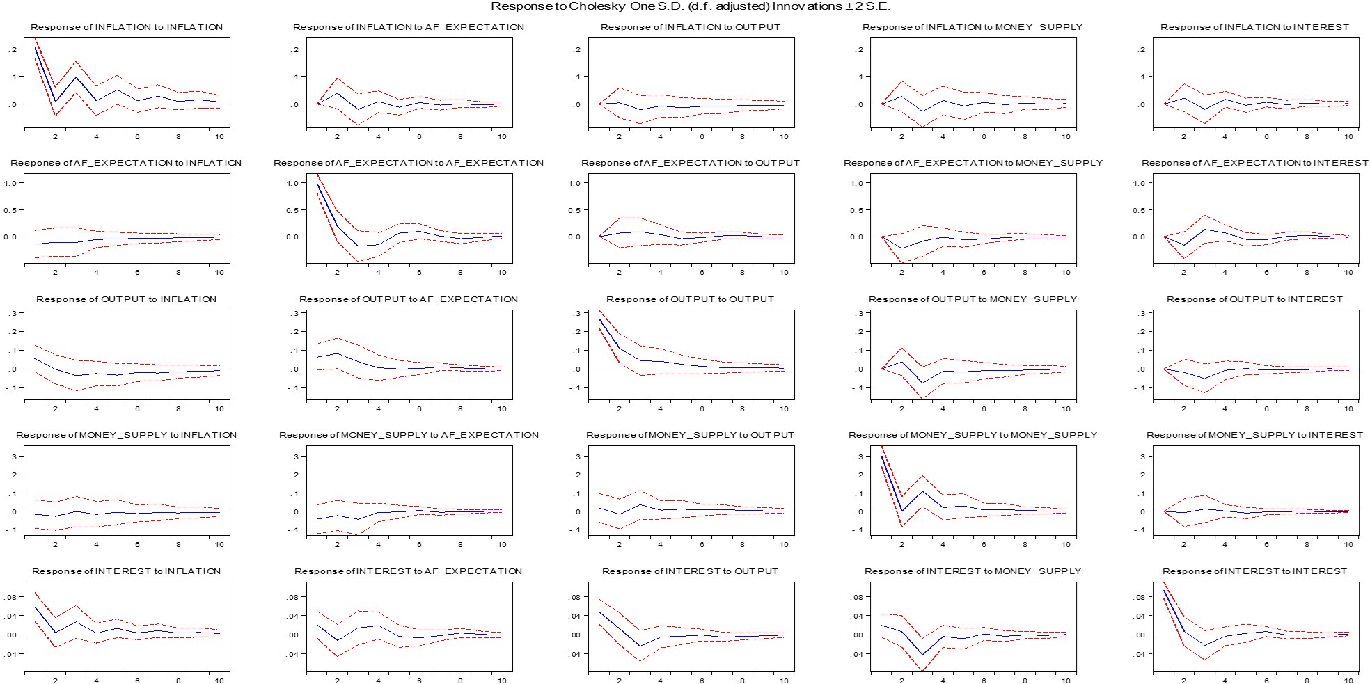
In Figure 1, we see that Cholesky decomposition is used and the order of identification is as follows: inflation, inflation expectations, output, money supply and interest rates. The second row of Figure 1 shows the response of inflation expectations to inflation, inflation’s own shock, output, money supply, and interest. A one standard deviation increase in inflation causes the expectations to gradually increase up till the fifth month and then the effect dissipates. An output shock leads to an increase in inflation expectations up to the second month; thereafter, it declines until it dissipates completely from the fifth month onwards. Inflation expectations increase slightly as output increases.

The money supply shock raises expectations for the second and subsequent months. Rising key interest rates will immediately lower inflation expectations in the Indian economy and, hence, a contractionary monetary policy is a well-thought-out decision by the central bank. This further helps build the credibility of the central bank, which helps foster economic development via better investments and lower inflationary expectations formation.

In the forecast error variance decomposition results, we see that 85 percent of the changes in expectations are self-explanatory in the long run implying that policymakers must be careful about raising expectations in the present as it would lead to persistent expectations in the future. Expectations are sticky downwards and are quick to rise.

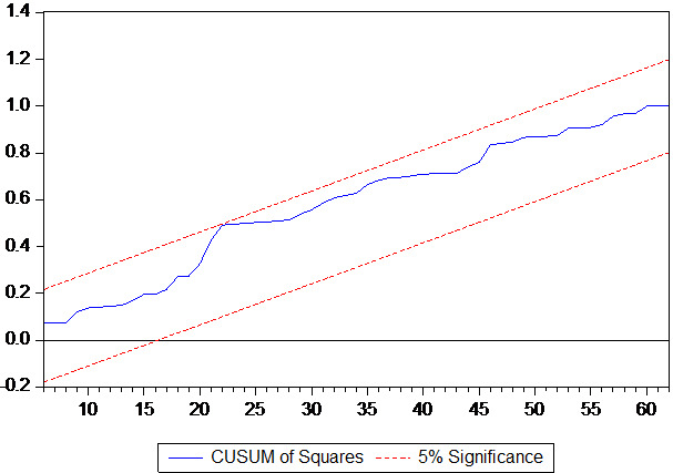
Since the model passes the Lagrange Multiplier autocorrelation and Whites heteroscedasticity, and cumulative sum of squares stability tests, our results are valid for meaningful interpretation.

Figure 1.Impulse Response Functions

This figure reports impulse responses with full VAR lag structure. Model is estimated using monthly Indian data from June 2016 - 2017 till September 2021 - 2022. Impulse responses are given by the solid lines. Dotted lines represent 0.68 error bands. Shock 1 is a one standard deviation shock to inflation. Shock 2 is a one standard deviation shock to inflation expectations. Shock 3 is a one standard deviation shock to output. Shock 4 is one standard deviation shock to money Supply. Shock 5 is one standard deviation shock to interest rates.

Figure 2.Stability tests

This figure plots CUSUM of Squares Stability Test and passes the test at five percent significance levels. Hence, the model coefficients are stable in the long-run.

IV. Conclusion

The motivation behind this work was to analyse the impact of monetary policy expectations channels. We see that inflation and money supply will rise as expectations rise, while interest rates and real output will fall. As money supply grows, expectations fall at first, but later rise within boundaries. Therefore, increasing money supply to cushion output decrease is a prudent decision by the central bank in times of crisis. Also, expectations fall instantly with a contractionary monetary policy of rising interest rates.

These results provide a solid explanation of India’s monetary policy expectations channel, as this is the best inflation forecast data possible. In addition, expectations can become an even more important variable in the coming years, making it important for central banks to build trust through communication and appropriate policy responses. With this new approach, one may continue to investigate the performance of the expectations channel. However, for a proactive policy approach, a solid forecast of future expectations is important. This further calls for a review of all the approaches that central banks around the world have adopted to create the best possible approach.

To anchor better expectations, we suggest that the RBI develops its own mobile app for the public and conduct direct local and urban surveys to better use this data to develop policies. As rightly said, “Data is king”, especially real-time data.

Appendix