The Feldstein-Horioka Puzzle in India: Some Asymmetric Evidence

I. Introduction

During the last three decades, the world has witnessed a tremendous increase in capital mobility. This increased cross-border capital mobility has helped economies to achieve higher investment, which further led to higher economic growth (Dash, 2019). Further, an economy can borrow from the international financial markets to finance its investment demand and achieve higher growth even in the presence of lower domestic savings (Garg & Prabheesh, 2017). Thus, domestic savings need not be converted into domestic investment as the savers have the best opportunities to invest their funds across the globe. However, the positive correlation between the domestic savings and investment contradicts the idea of international perfect capital mobility. In this context, the seminal work by Feldstein and Horioka (1980) (FH, hereafter) regresses investment on saving to measure the relationship between saving and investment for 16 OECD economies over the period 1960-1974. The model takes the following form:

$${(\frac{I}{Y}}_{i}) = \alpha + \beta{(\frac{S}{Y})}_{i} + \varepsilon_{t} \tag{1}$$

where, the parameter $\beta$ shows the strength of the relationship between investment$\ (\ \frac{I}{Y}_{i})$ and saving $\ (\ \frac{S}{Y}_{i})$ for country $i$ and indirectly measures the degree of capital mobility. In the case of $\beta = 0,$ domestic saving and investment are uncorrelated, indicating perfect capital mobility. Conversely, if$\ \beta = 1,$ there is perfect capital immobility. Finally, if $0 < \beta < 1,$ it shows there is imperfect capital mobility. Their empirical analysis obtained a value of $\beta$ close to 1 among OECD countries. This resulted in a “puzzle”, as there is a high correlation between domestic savings and investment in highly integrated economies, which is popularly known as the FH Puzzle.

From the empirical literature, mixed evidence has been reported. However, most of the studies found the value of $\beta$ between 0 and 1 (Dash, 2019; Fouquau et al., 2008). For instance, some studies found a higher value of the coefficient (Drakos et al., 2017), whereas some found a lower value of the coefficient (Ang, 2007; Kollias et al., 2008). This could be attributed to several factors like country size, home biasedness and substitutability of savings, information asymmetry, investor risk aversion, and differences in legal systems (Apergis & Tsoumas, 2009; Obstfeld & Rogoff, 2000). Indirectly, the coefficient represents how much domestic or foreign funds finance the domestic investment. Further, in a practical sense, it enables the assessment of the degree of capital mobility for an economy and is a suitable way of validating whether raising savings is the most efficient way of achieving higher investment (Dash, 2019).

With this background, we examine the savings-investment nexus in the case of India. Instead of the symmetric association largely assumed in previous studies, we explored the possibility of an asymmetric relationship since the response of investment to positive and negative changes in savings may not be uniform due to different macroeconomic circumstances or the investment characteristics like downward rigidity. We choose India as a case study because (1) India is a highly integrated economy to the outside world, but it is yet to enjoy the perfect capital account convertibility (Padhan & Prabheesh, 2020), (2) India is amongst the fastest-growing economies, and (3) the paramount importance has been given to savings and investment as a macroeconomic stabilizer in promoting employment and sustainable economic growth.

Our approach to examine the asymmetric savings-investment nexus is as follows. First, we choose India and collect data on gross domestic savings and investment over the period 1997Q1-2019Q2. Second, we employ a non-linear autoregressive distributed lag model (NARDL) model to investigate the asymmetric cointegration between savings and investment. Finally, we applied the Hatemi-J’s (2012) asymmetric causality test to uncover the possibility of asymmetric causality between partial sum decompositions of savings and investment. Our empirical findings are as follows: (1) the acceptance of the FH Puzzle for the Indian economy, which implies the presence of imperfect capital mobility, (2) the positive (negative) saving causes positive (negative) investment, and (3) negative (positive) saving does not cause positive (negative) investment.

We contribute to the literature on the following grounds. First, to the best of our knowledge, this is the first study to explore the asymmetric saving-investment relationship for the Indian economy. Second, we applied an asymmetric causality test to establish the causal interactions between the positive and negative sum decompositions of the two variables. Our analysis would enrich the existing literature with asymmetric linkages about the FH hypothesis.

The rest of the paper is organized as follows. Section II presents data and methodology. Section III provides the empirical findings. Section IV concludes our study.

II. Data and Empirical Methodology

We utilize quarterly data from 1997Q1 to 2019Q2. Saving and investment are proxied using gross domestic saving (S) and investment (I), respectively, both expressed as a percentage of gross domestic product and collected from the Handbook of Statistics on the Indian Economy, Reserve Bank of India.^[1] Simple correlation analysis indicated a high degree of positive association between domestic savings and investment, an earlier indication in favor of the FH puzzle. However, instead of a linear association, we test for the possibility of an asymmetric relationship.

To detect the long-run and short-run asymmetric relationship between saving and investment, we applied the NARDL model proposed by Shin et al. (2014). With the greater flexibility in relaxing the same order of integration assumption, it allows for a combination of I (0) and I (1) variables for the estimation. Further, it is a convenient approach, as it provides a dynamic error correction specification combined with an asymmetric long-run cointegration equation by decomposing a given time series into its oppositely signed partial sums. More importantly, it provides a solution to weak endogeneity, and if the lag structure is correctly chosen, it avoids the problem of autocorrelation. Finally, asymmetry switching is permitted wherein the positive shock may have a stronger effect in the short-run and the negative shock may be pronouncing in the long-run.

Thus, our asymmetric model specification takes the following form:

$$\begin{align} \mathrm{\Delta}I_{t} &= \ \alpha + \gamma\mathrm{\Delta}I_{t - 1} \\ &\quad + \delta_{1}^{+}S_{t - 1}^{+} + \delta_{1}^{-}S_{t - 1}^{-} + \sum_{i = 1}^{m}{\pi_{i}{\mathrm{\Delta}I}_{t - 1}} \\ &\quad + \sum_{i = 0}^{n}{\beta_{i}^{+}\mathrm{\Delta}S_{t - 1}^{+}} + \sum_{i = 0}^{n}\beta_{i}^{-}{\mathrm{\Delta}S}_{t - 1}^{-} + \mu_{t} \end{align} \tag{2}$$

where $S$ and $I$ are defined above. The parameters $\delta_{1}^{+}\ and\ \delta_{1}^{-}$ are long-run asymmetric coefficients, $\beta_{i}^{+}\ \ and\ \ \beta_{i}^{-}$ are short-run asymmetric coefficients, and $\mu_{t}$ is the white noise error term. First, the existence of cointegration is tested by using the bounds $F_{PSS}$ test and $t_{BDM}$ test. For asymmetric investigation, this specification incorporates several possibilities: (i) there is no short-run asymmetry, $\sum_{i = 0}^{n}\beta_{i}^{+} = \ \sum_{i = 0}^{n}\beta_{i}^{-},$ (ii) there is no long-run asymmetry, $\delta_{1}^{+} = \ \delta_{1}^{-},$ and (iii) there is neither short-run nor long-run asymmetry. Wald test having a null hypothesis of symmetrical association is tested against an alternative hypothesis of asymmetrical association in both the short- and long-run. Finally, the cumulative dynamic multipliers portray the traverse from any short-run distortion to the new long-run equilibrium position.

Finally, we applied an asymmetric causality test developed by Hatemi-J (2012) to explore the asymmetric direction of causality between positive and negative-sum decompositions of saving and investment. Further, a bootstrap simulation approach with leverage adjustment is used to generate critical values that are robust to non-normality and time-varying causality.^[2]

III. Empirical Findings

We started with time series properties of the variables using Augmented Dickey-Fuller (ADF) and Kwiatkowski-Phillips-Schmidt-Shin (KPSS) unit root tests. The results show S is I (1) and I is I (0).^[3] The mixed order of integration is suitable for NARDL analysis.

The results obtained from estimating Equation (2) are reported in Table 2. A general to specific approach is adopted to select the appropriate model. Initially, a lag length of max $p = q = 4$ is selected according to AIC and SBC criteria. However, most of the insignificant lags are dropped to avoid noise in the cumulative dynamic multipliers. Panel B of Table 2 documents evidence in favor of long-run cointegration because both $F_{PSS}$ and $t_{BDM}$ tests are statistically significant. The necessary diagnostic tests of estimated model are given in Panel C.

Having confirmed the long-run association, we switched to Wald’s test results for asymmetry analysis. Panel A depicts evidence of long-run asymmetric association. However, in the short-run, the null of symmetry cannot be rejected.

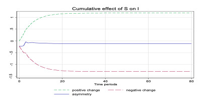
In the long-run, the relationship between investment and savings is found to be positive. However, the impact of the increase in savings is found to be markedly different from the decrease in savings. Specifically, a 1% increase in savings rate leads to a 1.182% increase in investment whereas a 1% decrease in savings lowers the investment by 1.298%. The outcome of this result highlights the validity of the FH puzzle and a case of imperfect capital mobility in India. Given the imperfect capital mobility on the capital account of the balance of payments, this result appears to be convincing. The results are in line with Yilanci and Kilci (2021) and Pata (2018).

Usually, savings rise during boom periods wherein the growth of incomes is positive. When the domestic savings increase in the economy, it implies more availability of funds in the market, a lower interest cost and therefore more investments to take advantage of low-cost savings and demand pressures for goods and services. Conversely, a fall in savings would denote a falling income scenario and a lower demand in the economy. As a result, the response of investors would not be very encouraging. In the short-run most of the coefficients are statistically insignificant and are therefore left undiscussed. Finally, the cumulative effect of saving on investment is shown in Figure 1, exhibiting the asymmetric persistence in the long-run.

Figure 1.Cumulative Dynamic Multipliers

Figure 1 exhibits the traverse from any short-run distortion to new equilibrium in long-run.

In Table 3, Hatemi-J’s causality test shows that the null hypothesis that positive (negative) saving does not cause positive (negative) investment is rejected. This indicates the presence of causality between positive and negative sum components of variables; hence they improve the predictability of each other. However, we see that the null hypothesis that negative (positive) saving does not cause positive (negative) investment cannot be rejected, implying no cross causal relations. The causality pattern again establishes evidence in favor of the FH puzzle like Raza et al. (2018).

IV. Conclusion

This study examines the asymmetric saving-investment relationship for the Indian economy. Using the NARDL and Hatemi-J asymmetric causality test, we find the validity of the FH puzzle for the Indian economy, which is in line with the incomplete capital account convertibility and presence of financial constraints. Further, the positive (negative) saving causes positive (negative) investment, and negative (positive) saving does not cause positive (negative) investment. Overall, this study finds evidence of an asymmetric relationship between saving and investment for the Indian economy. Our results suggest that appropriate policies should be designed to promote the saving rate in the economy to ensure a sustained growth immune from erratic capital movements across economies. Future research can focus on examining the FH hypothesis during the COVID-19 pandemic, which causes financial instability across economies.