Market Efficiency and Volatility Persistence of Green Investments Before and During the COVID-19 Pandemic

I. Introduction

The clamor for a low-carbon economy to support friendly environmental projects to alleviate the negative effects of climate change led to the introduction of green investments and, since 2007, their markets have grown from $0.8 billion to $257.7 billion in 2019 (Climate Bonds Initiative, 2019; Hammoudeh et al., 2020). The launch of “Principles of Green Bond” by the International Capital Markets Association in 2014 further created more awareness of green bonds and green stocks among scholars, investors, and policymakers. Green investments are known to be useful in rating a low carbon economy (Larcker & Watts, 2019), and for reducing global coal consumption leading to low CO₂ emissions (Glomsrød & Wei, 2018).

Green finance is a future-oriented type of finance that targets the financial industry by improving the environment and enhancing economic growth due to its low-carbon initiative. The current COVID-19 pandemic has affected global finance, quite more than the global financial crisis of 2008/09, with the market fearing more during the health crisis (Yaya et al., 2021). The pandemic led to the further disentanglement of international financial markets, which affected the level of market integration. Quite several papers investigate the impact of the pandemic on financial markets (Darjana et al., 2022; Salisu & Sikiru, 2020), and on energy and oil (Narayan, 2020), among others. The global concern on green finance for economic growth is growing rapidly amid economic and geo-politically-induced uncertainties (Adekoya et al., 2022), particularly the current global health concern as it imparts on green investments.

This paper, therefore, investigates the level of market efficiency and volatility persistence of green investments before and during the COVID-19 pandemic, using a two-year daily data window in each case. While the determination of market efficiency will render useful information for market players in terms of the possibility of trading for excess gains (Gil-Alana et al., 2018; Yaya et al., 2021), the assessment of volatility persistence will help policymakers to know how best to tackle market disruptions caused by a one-time shock to keep the green investment market in shape towards the fulfillment of its environmental sustainability objective. Fractional integration techniques are employed on the datasets to test: (a) the white noise hypothesis in prices and returns; and (b) the persistence in absolute returns used as a proxy for volatility in the series. Thus, market efficiency in price series requires that price series are $I(d = 1)$ as in the case of random walk, which further implies that the first differences of price series (i.e. the log-returns) are $I(d = 0).$ Evidence of market inefficiency, thus, means that $I(d < 1),$ which is the case of long-range dependency of the series.

II. The $I(d)$ model for testing market efficiency

The persistence analysis conducted in this paper is based on Cuestas and Gil-Alana’s (2016) nonlinear $I(d)$ framework. The authors introduced the Chebyshev polynomials in time to the fractionally integrated model of Robinson (1994) to form a non-linear deterministic test for testing non-linearity in $I(d)$ processes. The setup of the test is as follows. Consider a general model,

$$y_t=f\left(\theta ; z_t\right)+x_t, \quad t=1,2, \ldots, \tag{1}$$

where $y_t$ is the observed time series and $x_t$ follows an $I(d)=(1-L)^d$ process, with $x_t = 0$ for $t \leq 0$ and $d>0$ where $L$ is the lag-operator $(Lx_t=x_{t-1})$ and $u_t$ is $I(0)$ series. The function $f(.)$ is a non-linear function that depends on the unknown parameter vector of dimensions $m,\ \theta,\ z_{t},$ which is a vector of deterministic terms. Then, Eq. (1) can be re-written as,

$$y_t=\sum_{i=0}^m \theta_i P_{i, N}(t)+x_t, \quad t=0, \pm 1, \ldots, \tag{2}$$

where the order of the Chebyshev polynomial is m. The Chebyshev polynomial $P_{i, N}(t)$ in Eq. (2) is defined as,

$$\begin{align} P_{i, N}(t)&=\sqrt{2} \cos [i \pi(t-0.5) / N], \\ t&=1,2, \ldots, N ; i=1,2, \ldots, \tag{3} \end{align}$$

with $P_{0, N}(t)=1$. From the polynomial, whenever m = 0, the model is expressed with an intercept only; if m = 1, it contains an intercept and a linear trend, and when m > 1, it becomes non-linear, and the higher m is the less linear the approximated deterministic component becomes. The choice of value for m then depends on the significance of the Chebyshev coefficients.

The non-linear deterministic approach of long-range dependence by Chebyshev polynomials is a modification and improvement of Robinson’s (1994) fractional integration technique. Robinson (1994) considers the same setup as in Eqs. (1) and (2) with $f(.)$ in Eq. (2) of the linear form, $\theta^{\prime} z_t$, testing the null hypothesis,

$$H_0: d=d_0, \tag{4}$$

for any real value $d_0$. Under $H_0$ and using the two equations,

$$y_t^*=\theta^{\prime} z_t^*+u_t, \quad t=1,2, \ldots, \tag{5}$$

where $y_t^*=(1-L)^{d_0} y_t$ and $z_t^*=(1-L)^{d_0} z_t$. Then, given the linear nature of the above relationship and the $I(0)$ nature of the error term $u_t$, the coefficients in Eq. (5) can be estimated by standard Ordinary Least Square (OLS) or Generalized Least Squares (GLS) methods. The same applies to the case of $f(.)$ containing the Chebyshev polynomials, noting that the relationship is linear in parameters. Thus, combining Eqs. (1) and (3), we obtain,

$$y_t^*=\sum_{i=0}^m \theta_i P_{i, N}^*(t)+u_t, \quad t=0, \pm 1, \ldots, \tag{6}$$

where $P_{i, N}^*(t)=(1-L)^{d_0} P_{i, N}(t)$and using OLS/GLS methods, under the null hypothesis in (4), the residuals $\hat{u}_t$ are,

$$\begin{align} \hat{u}_t&=y_t^*-\sum_{i=0}^m \theta_i P_{i, N}^*(t) ; \\ \hat{\theta}&=\left(\sum_{t=1}^N P_t P_t^{\prime}\right)^{-1}\left(\sum_{t=1}^N P_t y_t^*\right), \tag{7} \end{align}$$

and $P_t$ is the $(m \times 1)$ vector of Chebyshev polynomials. Based on the above residuals $\hat{u}_t$, we estimate the variance,

$$\hat{\sigma}^2(\tau)=\frac{2 \pi}{N} \sum_{j=1}^N g\left(\lambda_j ; \hat{\tau}\right)^{-1} I_{\hat{u}}\left(\lambda_j\right) ; \quad \lambda_j=\frac{2 \pi j}{N}, \tag{8}$$

where $I_{\hat{u}}\left(\lambda_j\right)$ is the periodogram of $\hat{u}_t$; $g$ is a function related to the spectral density function of $u_t$; and the nuisance parameter $\tau$ is estimated by $\hat{\tau}=\arg \min _{\tau \in N^*} \sigma^2(\tau)$, where $N^*$ is a suitable subset of the $R^{q}$ Euclidean space.

III. Data and Empirical Results

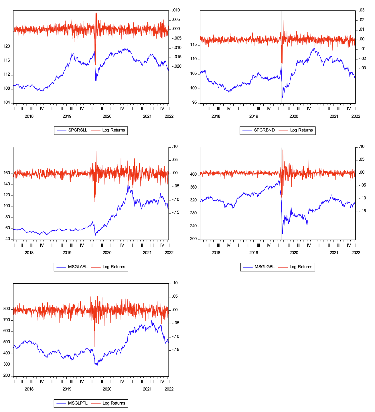
We obtain daily data on green investments from Datastream. We consider a two-year data window before the COVID-19 pandemic, i.e. before the World Health Organization’s pandemic declaration date of 11 March 2020, and another two-year data window after this date. Thus, the entire sample analyzed spans 1 March 2018 to 13 January 2022. Five green investment indices, i.e. bonds and stocks, are analyzed. The green bond indices are the S&P Green bond select index (SPGRSLL), and the S&P Green bond index (SPGRBND), while the green stock indices are the Morgan Stanley Capital International (MSCI) global alternative energy index (MSGLAEL), MSCI global pollution prevention index (MSGLPPL), and the MSCI global green building index (MSGLGBL). The MSCI indices for green investments take up about half of the revenue from securities on environmental-friendly projects, such as those of green building, alternative energy, clean water, or pollution prevention. Thus, the five variables analyzed in this paper represent global green investments.

Plots of prices of these green investments are given in Figure 1 with the corresponding log-returns superimposed. The green assets are seen to exhibit significant volatility in both prices and returns, with stronger evidence since 2020. The relative stable trend enjoyed by the assets at the beginning of the sample period halted with a sharp drop in their prices around the first quarter of 2020, coinciding with the period when the pandemic outbreak news peaked (Umar et al., 2021).

Figure 1.Plots of price and log-returns of Green investments

We start the main results with the logged prices, as reported in Table 1. the d estimates for both green bond indices, SPGRSLL (1.0117) and SPGRBND (0.9943), are not significantly different from unity before the COVID-19 pandemic, implying that the null hypothesis of random walk, which is consequently associated with market efficiency, cannot be rejected. This is unlike other green assets whose d estimates exceed one. During the pandemic, however, the green bond market tends to lose its efficiency in favour of persistence, following an increase in the d estimates of both green bond indices beyond the region of d = 1. Other green assets still maintain their initial status, except the global green building index (MSGLGBL), which is now demonstrating a random walk, given its d estimate is 1.0123.

We next turn to the log-returns and volatility (absolute returns) results. The consideration of volatility persistence is an extension of the conventional weak-form efficiency hypothesis that merely relies on asset prices or returns. Volatility persistence is important in determining how long-lasting the effect of shocks that increase the riskiness of a financial asset would be. As shown in Tables 2 and 3 for the log-returns and volatility results, respectively, the significance of the fractional parameter, d, tends to vary for some assets both across the series (returns and volatility) and periods (before and during the pandemic). Nonetheless, significance is established in most cases, and there is clear evidence that the estimates of d fall in the 0<d<0.5 range. This suggests that the green assets’ returns and volatilities demonstrate long memory and mean-reverting features. Therefore, the effect of shocks will only be transitory, dying out in no distant time. Besides, the values of d seem to be greater during the pandemic, as an indication that the rate at which it will die out will be slower in this period. This is consistent with the finding of Adekoya et al. (2021) that the green bond market shows evidence of stronger persistence during the pandemic. One probable reason for this is that, apart from the pandemic affecting the individual financial market, it resulted in significant risk transmissions, induced high fear and pessimism in investors (Umar et al., 2021), and erratic speculative behaviour. Based on these factors, adjusting to a normal market state could require a longer recovery time.

IV. Conclusion

This study examines the market efficiency and volatility of green investments before and after the COVID-19 pandemic. Using fractional integration methods, we find that the green bond market, which was efficient before the pandemic, demonstrates inefficiency during the crisis. However, other green markets are inefficient in both periods, except for MSGLGBL. In addition, the green assets’ returns and volatilities are found to observe mean-reverting behaviour, indicating that the effect of shocks will be temporary, although will die out more slowly during the health crisis.

Green investors can glean from these findings that they can make abnormal profits following the inefficient states of the markets, except for green bonds during tranquil periods. However, they should be aware that any shock that adversely affects returns during a similar crisis will have a relatively slower time of disappearance unlike when the market is normal.