The Road to Improve Energy Efficiency vs. the Role of Corruption: A Dynamic Quantile Exploration

I. Introduction

The incidence of corruption in the business environment can influence energy efficiency (EE) both directly and indirectly. Corruption affects firm performance directly by constraining or favoring growth-improving production activities. Indirectly, corruption may condition the degree of efficiency with which production factors are reallocated across firms operating in a given industrial sector, by channeling or diverting resources from the most to the least productive production units.

The macroeconomic effect of corruption is well addressed in the literature. Empirical findings show mixed conclusions, supporting both the view that: (1) corruption has the potential to boost economic development in that it constitutes the necessary “grease” to lubricate the stiff wheels of rigid government supervisors and the legal systems; and that (2) the rent-seeking behaviour of corrupt government officials may hinder economic development, as illustrated by “sanding-the-wheel” advocates.

The Chinese economy is dominated by the government, which maintains control over key production resources and determines resource allocation (Guo et al., 2021). Firms with political connections and state-owned enterprises may receive favorable treatments through various channels, such as subsidies and special low-interest rates. Therefore, in an economy plagued with corruption, firms are willing to engage in more rent-seeking activities and to establish political connections with the government to obtain scarce resources. Still, if resources are channeled according to the political connections and ownership, then state-owned enterprises and politically connected firms with lower productivity will obtain more market resources than other firms with higher productivity.

Besides, China’s “local protectionism” is also heavy, which prevents labour and capital resources flowing freely between economic zones. Factors of production cannot operate in accordance with the economic operation laws of entering regions with low marginal productivity into regions with higher marginal productivity, which results in inefficient allocation of production factors, triggers capital and labour misallocations, thereby damping EE. (Hao et al., 2020). Therefore, a dynamic panel quantile regression (DPQR) model^[1] addressing possible endogeneity issue is employed by this paper to model the effect of corruption on EE.

II. Materials and Data

We employ the DPQR model with fixed effects proposed by Galvao (2011) as our benchmark regression model. Consider the following classic dynamic panel data model:

$$y_{it} = \alpha_{i} + \beta y_{it - 1} + x_{it}^{'}\gamma + \varepsilon_{it}\tag{1}$$

where $y_{it}$ represents the EE in province $i$ for year $t;$ $y_{it - 1}$ is the lagged dependent variable; $x_{it}$ denotes the selected control variables, including the core explanatory variable, corruption, determined by the number of the number of cases of malpractice tort crime, and the investigation of the crime of embezzlement and bribery cases on file (lncor), fdi proxied by foreign direct investment actually utilised to gross domestic product (GDP), economic growth represented by per capita GDP (lnpgdp), industrialisation rate (ir) expressed by the ratio of industrial value added to GDP, industrial structure upgrading measured by the share of tertiary output to secondary output (isu), and technological innovation expressed by the number of patent granted (lnpat). $\alpha_{i}$ is the province specific effect; and $\varepsilon_{it}$ is the error term.

Considering the varying influence of corruption on EE, the analogous version to Eq. (1) for the $\ell^{th}$ conditional quantile functions of the response to the $\ell^{th}$ observation on the i-th individual $y_{it}$ is specified as:

$$Q_{y_{it}}\left( \ell \middle| y_{it - 1,\ }x_{it} \right) = \alpha_{i} + \beta\left( \ell \right)y_{it - 1} + x_{it}^{'}\gamma\left( \ell \right)\tag{2}$$

In Eq. (2), the effects of the covariables $(y_{it - 1},x_{it})$ depend on the $\ell^{th}$ conditional quantile. The individually unobservable heterogeneity will be captured by $\alpha_{i}.$ Galvao (2011) uses higher-order $y_{it}$ as instruments to attenuate the bias and generate consistent estimators that are independent of initial conditions learnt from Anderson & Hsiao (1982) and Bond (1991), when estimating of the DPQR model. Specifically, he uses instruments $\kappa_{it}$ that correlate with $y_{it - 1},$ but which are independent of $\varepsilon_{it}.$ Thus, the objective function is given as follows:

$$\small{ \min_{\beta,\gamma,\alpha}{\sum_{t = 1}^{T}{\sum_{n = 1}^{N}\theta_{\ell}\left( y_{it} - \alpha_{i} - \beta\left( \ell \right)y_{it - 1} - x_{it}^{'}\gamma\left( \ell \right) - \psi\left( \ell \right)\kappa_{it} \right)}}} \tag{3}$$

where $\theta_{\ell}(\mu)\ = \mu(\ell - I(\mu < 0))$ is the quantile loss function.

Suggested by Chernozhukov & Hansen (2006), two-ordered lagged $y_{it}$ is treated as instrument. Subsequently, we first define a grid of values $\left\{ \beta_{j},j = 1,J;|\beta| < 1 \right\}.$ And then we regress the ordinary quantile regression with fixed effects of $y_{it} - \beta\left( \ell \right)y_{it - 1}$ on ${(\alpha}_{i},\ x_{it},\kappa_{it})$ to minimise Eq. (3) for $\alpha,$ $\gamma$ and $\psi$ following Galvao (2011). Lastly, we use the value of $\overline{\beta}(\ell)$ to minimise the objective function below:

$$\overline{\beta}\left( \ell \right) = arg\min_{\beta_{j}}\left\lbrack \overline{\psi}\left( \beta_{j},\ell \right)^{'}B\overline{\psi}\left( \beta_{j},\ell \right) \right\rbrack\tag{4}$$

where $B$ represents the positive definitive matrix. We compute Eq. (4) using the grid method and treat matrix $B$ as the identity matrix. In other words, $\overline{\beta}$ is used when it results in the minimum square of $\overline{\psi}\left( \beta_{j},\ell \right).$ Once the optimal $\overline{\beta}\left( \ell \right)$ is identified, the quantile regression with fixed effects of $y_{it} - \beta\left( \ell \right)y_{it - 1}$ on ${(\alpha}_{i},\ x_{it},\kappa_{it})$ to derive the coefficients of $\overline{\beta}\left( \ell \right)$ is determined. Thus, consistent estimates of $\left\lbrack \overline{\beta}\left( \ell \right)\overline{\gamma}\left( \ell \right) \right\rbrack$ are obtained.

The core of the estimation mentioned above is that the coefficients of the instruments equal zero once the instrument utilised is valid (Chernozhukov & Hansen, 2006). We can get a consistent estimate of the lagged $y_{it}$ by minimising the instrument’s coefficient. Additionally, the dynamic bias caused by the lagged $y_{it}$ can drop in the presence of effective instruments (Galvao, 2011). The bootstrapped robust standard errors are derived by performing Monte Carlo simulations with 500 replications.

Following Li & Lin (2015), a sequential DEA model is performed to measure EE levels in China. Specifically, capital, labour, and total energy consumption are treated as input factors. Real GDP is selected as desirable output, while CO₂ emissions are considered as undesirable output. Among which, capital stock is calculated adopting the perpetual inventory method. CO₂ emissions are calculated following the Intergovernmental Panel on Climate Change report in 2006 and the fossil fuel consumption released by the National Development and Reform Commission in 2007.

A panel data from 30 Chinese provinces spanning 1998-2016 is used to examine the effect of corruption on EE. The data come from China Energy Statistics Yearbook, Wind database, and China Statistical Yearbook. The GDP values are deflated to 1998 constant prices. Total investment in fixed assets has been deflated using price index for investment in fixed assets. Descriptive statistics of all selected variables and unit-root test results are documented in Table 1.

III. Findings

According to Fig. 1, EE levels in most Chinese provinces show a significant upward trend (albeit with small fluctuations in some provinces like Guangxi). Second, compared with some eastern provinces, the western provinces (e.g., Inner Mongolia) still lagged. Third, EE performance in some eastern coastal provinces (e.g., Guangdong and Shanghai) is better than that of other provinces (e.g., Tianjin and Hebei). In conclusion, there is a greater room for China to simultaneously reduce CO₂ emissions and improve eco-efficiency.

Figure 1.EE spatial distribution.

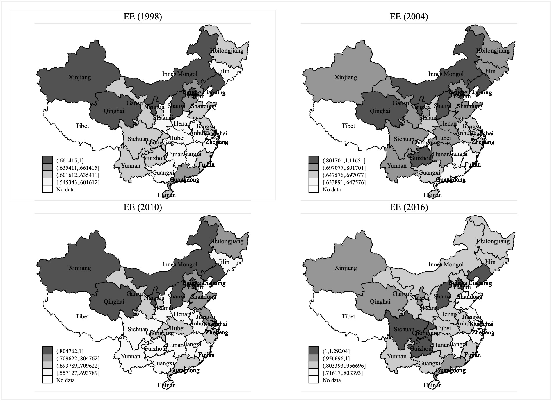
Table 2 reports the effects of corruption on EE using the DPQR model. For comparison, the first differenced generalised method of moment (GMM) and system GMM results are also reported.

In general, the influential impact of corruption on EE has decreased at the conventional level of statistical significance in the median and upper quantiles of the distributions, creating an “M-shaped” trend. The empirical studies confirm that corruption dampens the strictness and completeness of environmental and energy policies. It could increase air pollution, deforestation, and restrict the allocation of public goods (i.e., public facilities), affect the ratification of the Kyoto protocol (Barbier et al., 2005; Biswas et al., 2012). That is, the higher the level of corruption, the greater the degree of resource misallocation (Wang et al., 2020).

When the carbon compensation markets and carbon emissions in China cannot be effectively regulated, the government’s response to correct and guide abuse will make potential issues persistent and worse. These regulatory actions will pose a threat to social development (Lohmann, 2009). An increase in the share of official corruption may weaken environmental regulation, resulting in increased illicit production and pollution emissions (Chen et al., 2018). Moreover, the distortion of resource allocation triggered by corruption may lead to inefficiency issues (Yang et al., 2018). Additionally, the lower quantile regression coefficient is slightly higher than that of higher quantile, implying that for some Chinese provinces with low EE values, corruption causes more pollution emissions and reduces EE.

The lagged explained variable is statistically positive and significant at the 1% significance level in all models, implying that the past accumulation of EE is highly correlated with the current EE improvement; thus, the “accumulation effect” of EE is identified.

There is evidence of regional heterogeneity of corruption’s effect on EE. According to Table 3, corruption significantly inhibits EE in the eastern region, excluding in the upper quantile. In contrast, the inhibitory effects are relatively weaker in the central (or even positive at the 0.3 quantile) and western regions. These results imply that severe corruption could significantly curb EE in the eastern region.

Corruption generally means social and political problems triggered by improper behaviour and work types of public officials associated to social and economic development. High-polluting firms lobby the local government through political donations to reduce the stringency of environmental regulations (Dincer & Fredriksson, 2018); thus, collusion between business and government occurs. The “benefits” force officials to provide investors with an opportunity to “take loopholes”. Consequently, inefficient environmental supervision or law enforcement can lead energy-intensive and high-polluting firms to move to the local area, such that it becomes a “pollution paradise”. Therefore, it is necessary to strengthen environmental management and administrative efficiency of the local government, especially in both the central and western regions.

IV. Conclusions

We employ panel data of 30 Chinese provinces spanning from 1998 to 2016 to shed new light on the effect of corruption on EE from the national and regional perspectives. We find that: (1) there is an evidence of imbalance across provinces concerning EE performance; and (2) corruption significantly curbs EE at the national level, while the inhibitory effects exhibit regional heterogeneity. Finally, two policy implications are derived: (1) the government should enhance regional factor (i.e., labour and capital) flow mechanisms and reduce flow costs. That is, a regional sharing mechanism should be established to improve economic efficiency in the central and western regions; and (2) the government should strongly carry out anti-corruption campaign, uphold integrity, and improve environmental management efficiency.