The Predictive Power of Monetary Policy on International Stock Market Returns—Evidence From TV-ARMAX Model

I. Introduction

The evolution of methodology employed to study the relation between monetary policy and stock market returns can be summarized as follows. Early studies used linear regression (e.g., Bernanke & Kuttner, 2005; Patelis, 1997). Later studies (e.g., Bernanke et al., 2005; Bjørnland & Leitemo, 2009) use VAR and its variants to recognize the interdependence between market returns and monetary policy. Also, some papers apply the nonlinear models, such as the nonlinear VAR model (Sun & Wang, 2018) and the STAR-X model (Dahmene et al., 2021). Most recently, researchers have started to use time-varying coefficient to study the relation (e.g., Cepni & Gupta, 2021).

Acharya et al. (2020), Dahmene et al. (2021) and Bianchi et al. (2022) find that monetary policy affects the stock market diversely at different times. However, there have been very few attempts that allow time-varying coefficient of the input variables while outlier events (e.g., the financial crisis and European debt crisis) may distort coefficient estimates which add to prediction error. Our TV-ARMAX model fills this gap by allowing time-varying coefficient estimates and filtering outlier data points. Moreover, as documented by Anarkulova et al. (2022), phenomena observed in the US market – the most prevailing market in which prior research conducts empirical tests – may not hold in other markets. Therefore, our paper validates models on a multi-country base.

This study contributes to the literature by addressing the above issues, which seem to have received only limited attention (if any at all) from prior studies. Particularly, we employ the time-varying ARMA model with exogenous variable (TV-ARMAX) and conduct tests across 31 countries for empirical practice.^[1] On the one hand, TV-ARMAX allows time-varying coefficients to capture the potential changes of effect over time. On the other hand, TV-ARMAX uses time-variant penalty which prevents periodic outlier events from distorting coefficient estimates. Finally, conducting tests from a wide range of countries gives strong support for the validity of our method as any findings made do not come from one single country.

Consistent with prior studies, we find that interest rate (a commonly used proxy for monetary policy) is negatively correlated with future market returns on average. Moreover, we observe time-varying effect of interest rate with the Global financial crisis and European debt crisis witnessing the highest effect of interest rate. In the out-of-sample prediction, our approach robustly outperforms other predictive models including the simple linear regression model (SLM), the vector autoregression (VAR), the VAR with exogenous variable (VARX), the time-varying vector autoregression (TV-VAR), and the ARMAX among both developed and emerging markets. Across all three settings – all markets, developed markets, and emerging markets – the prediction error of TV-ARMAX is only a small fraction of that of other models, indicating the superiority of our approach.

II. Methodology

A. The TV-ARMAX Methodology

TV-ARMAX model extends the ARMAX model by allowing the coefficient to vary with time and by adding a time-dependent cumulated variation penalty from Zhang et al. (2020). Given a time series $y_{t}$, for $t = 1,2,\ldots,T$, the dependent variable under TV-ARMAX (p, q, m) model is given by Eq. (1):

$$\small{y_{t} = \mu_{t} + \sum_{i = 1}^{p}\phi_{it}y_{t - i} - \sum_{j = 1}^{q}\theta_{jt}\epsilon_{t - j} + \sum_{k = 1}^{m}\beta_{kt}x_{t - k} + \epsilon_{t}}\tag{1}$$

In the equation above, $\mu_{t}$ is the drift term, $x_{t}$is the exogenous variable, $\phi_{t}$, $\theta_{t}$, and $\beta_{t}$ are coefficients, and $\epsilon_{t}$ is the independent $N(0,\sigma^{2})$ error term. Note that at time t, $y_{1}$, $y_{2}$, …, $y_{t - 1}$ are observable, and therefore we can define the error terms as:

$$\begin{aligned} {{\widehat{\epsilon}}_{t}}^{(T)}(\theta,\beta,\phi) &= y_{t} - \mu_{t} - \sum_{i = 1}^{p}\phi_{it}y_{t - i}\\ & \quad + \sum_{j = 1}^{q}\theta_{jt}{\widehat{\epsilon}}_{t - j} - \sum_{k = 1}^{m}\beta_{kt}x_{t - k} \end{aligned}\tag{2}$$

Our target function – sum of squares with time-dependent cumulated variation penalty at time T is given by:

$$\begin{aligned} Q_{T} &= \sum_{t = 1}^{T}\left( \widehat{o}(\theta,\beta,\phi) \right)^{2} + \sum_{t = 1}^{T}{\lambda_{t}\left( \mu_{t} - \mu_{t - 1} \right)^{2}}\\ & \quad + \sum_{t = 1}^{T}{\sum_{i = 1}^{p}{\lambda_{t}\left( \phi_{it} - \phi_{i,t - 1} \right)^{2}}}\\ & \quad + \sum_{t = 1}^{T}{\sum_{i = 1}^{q}{\lambda_{t}\left( \theta_{it} - \theta_{i,t - 1} \right)^{2}}}\\ & \quad + \sum_{t = 1}^{T}{\sum_{k = 1}^{m}{\lambda_{t}\left( \beta_{kt} - \beta_{k,t - 1} \right)^{2}}} \end{aligned}\tag{3}$$

Define ${\phi_{1t}}^{(T)},\ldots,{\phi_{pt}}^{(T)},{\theta_{1t}}^{(T)},\ldots,{\theta_{qt}}^{(T)}$ and ${\beta_{1t}}^{(T)},\ldots,{\beta_{mt}}^{(T)}$ for $t = 1,2,\ldots,T$ as the solution of the minimization of $Q_{T}$. The hyperparameter$\lambda_{t} = \kappa t^{\alpha}$ is calibrated using a grid point search.^[2] For robustness purposes, we consider both the non-adaptive and adaptive methods for hyperparameter calibration. In the Adaptive method, $\kappa$ is selected from $(10^{0},\ 10^{0.3},\ 10^{0.6},\ \ldots,\ 10^{2.7},\ 10^{3})$ and $\alpha$ is chosen from $\alpha = \frac{1}{5} + \frac{8}{15}i$ for $i = 1,2,...,8,9$. Intuitively, smaller $\kappa$ and $\alpha$ place lighter penalty on the inter-period difference of coefficients, which allows a higher degree of intertemporal variation. Non-adaptive method, on the other hand, lets $\kappa > \infty$, which allows no intertemporal difference of the coefficients. Following Zhang et al. (2020), we use a real-time O(1) updating strategy for determining the best combination of (p, m, q, $\kappa$, $\alpha$). Please see Appendix A for details.

B. The Prediction Models

In this section, we introduce the empirical application details of the TV-ARMAX model together with all other benchmark models. These models include the simple linear-regression model (SLM), vector autoregression model (VAR, TV-VAR, and VARX), and ARMAX. SLM is the most straightforward model which is a natural starting point. VAR is the most widely used model in the literature which warrants its inclusion. We also enhance VAR by allowing time-varying coefficients (TV-VAR) and by introducing exogenous variables (VARX). Finally, we consider the time-invariant version of ARMAX to directly demonstrate the importance of allowing time-varying coefficients.

Particularly, the TV-ARMAX model takes this form:

$$\begin{aligned} RET_{t} &= \mu_{t} + \sum_{i = 1}^{p}\phi_{it}RET_{t - i} - \sum_{j = 1}^{q}\theta_{jt}\epsilon_{t - j}\\ & \quad + \sum_{k = 1}^{m}\beta_{kt}MPOLICY_{t - k} + \epsilon_{t} \end{aligned}\tag{4}$$

where $RET_{t}$ is the MSCI stock index returns of one specific country, and MPOLICY is monetary policy, which is proxied by interest rate (INTEREST).

The ARMAX model takes this form:

$$\begin{aligned} RET_{t} &= \mu + \sum_{i = 1}^{p}\phi_{i}RET_{t - i} - \sum_{j = 1}^{q}\theta_{j}\epsilon_{t - j}\\ & \quad + \sum_{k = 1}^{m}\beta_{k}MPOLICY_{t - k} + \epsilon_{t} \end{aligned}\tag{5}$$

Note that the key difference between the ARMAX and the TV-ARMAX is that the coefficients in ARMAX are not time-varying.

We consider three types of vector auto-regression models; they are the VAR, the time-varying VAR (TV-VAR), and the VAR with exogenous variable (VARX).

In particular, the VAR(p) model is given by,

$$Y_{t} = A_{1}Y_{\text{t-1}} + \ldots + A_{1}Y_{\text{t-1}} + \mu_{t}\tag{6}$$

where $Y_{t} = (RET_{t},MPOLICY_{t})$ and $A_{i}$ is a$2 \times 2$ coefficient matrices.

The TV-VAR(p) model is given by

$$Y_{t} = X_{t}\beta_{t} + A_{t}^{- 1}\Sigma_{t}\varepsilon_{t}\tag{7}$$

where $Y_{t} = (RET_{t},MPOLICY_{t}),X_{t} = I_{k} \otimes (y_{t - 1}',...,y_{t - s}')$.

The VARX(p,q) model is given by:

$$\begin{aligned} RET_{t} &= \mu + \sum_{i = 1}^{p}\phi_{i}RET_{t - i}\\ & \quad + \sum_{i = 1}^{q}\beta_{j}MPOLICY_{t - j} + \varepsilon_{t} \end{aligned}\tag{8}$$

and all the variables are defined the same as before.

Finally, we include the simple linear-regression model (SLM) which is given by

$$RET_{t} = \mu + \sum_{i = 1}^{p}\beta_{i}MPOLICY_{i} + \varepsilon_{t}\tag{9}$$

C. Data and Sample Construction

We collect MSCI country-specific stock market indexes as proxies of stock market returns. We use central bank policy rate from Data and Statistics in Bank for International Settlements (BIS) as the proxy for monetary policy. The central bank policy rate is the interest rate (in level form), which is used by the central bank to implement or signal its monetary policy stance.^[3] The data frequency in this paper is monthly and the sample period is from January 2006 to April 2020. We use the Levin-Lin-Chu unit-root test and find that stock market returns and interest rate are both stationary. Please see Table B1 in Appendix B for the summary statistics across all countries. Figure C1 in Appendix C provides the cross-sectional average of interest rate from 2006 to 2020.

III. Empirical Results

A. In-Sample Coefficient of TV-ARMAX

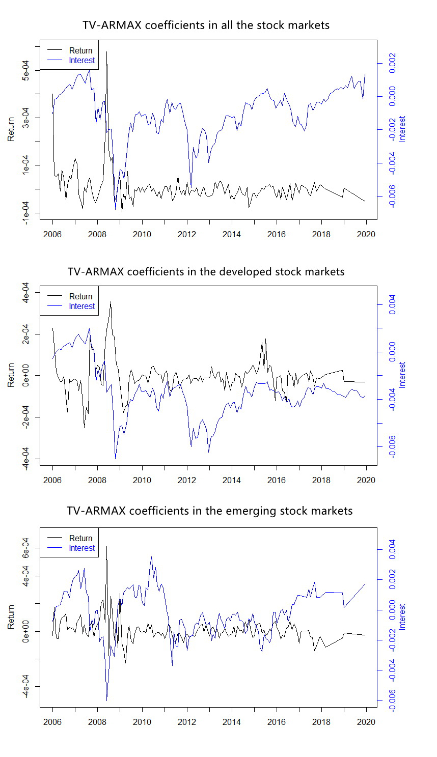
In this subsection, we apply the TV-ARMAX in Eq. (4) and obtain time-varying estimated coefficients for 31 stock markets. We calculate the cross-country average time-varying coefficients of the first lagged stock returns ($\phi_{t}$) as the optimal number and interest rate ($\beta_{t}$). Figure 1 plots the time series of cross-country averages for all stocks markets, developed stock markets, and emerging stock markets.

Overall, we observe apparent variation of the coefficient over time, which provides evidence for allowing time-variant coefficients of the model. During the Global financial crisis and European debt crisis, the negative impact of interest rate was at its highest since central banks in most countries applied an expansionary monetary policy in the recession periods and we tend to observe a sharp “bounce-back” of the stock market after sharp decreases of interest rates.

Figure 1.The cross-country average coefficients

Note: The cross-country average coefficients of first lagged stock return and interest rate using the TV-ARMAX model in all the markets, the developed markets and emerging markets.

B. Out-of-Sample Performance Using TV-ARMAX Model

In this subsection, we apply the TV-ARMAX model with non-adaptive method (TV-ARMAX_na), the TV-ARMAX model with adaptive method (TV-ARMAX_a), the ARMAX model, the VAR model, the TV-VAR model, the VARX model, and the simple linear model (SLM) for out-of-sample prediction. We calculate the average MSE, MAE and RMSE as measures of prediction error.^[4] We use the first 70% of the data as a training sample and apply the coefficients obtained to the remaining 30% of the sample for performance evaluation.

Panels A, B and C of Table 1 report the cross-country average performance in all markets, developed markets, and emerging markets, respectively. In all three settings, we find that TV-ARMAX methods generate meaningfully smaller prediction errors than models used in prior studies.^[5] We also observe that the adaptive version, TV-ARMAX_a, delivers a better performance than the non-adaptive version, TV-ARMAX_na.

To provide statistical evidence, we test the difference of prediction errors between TV-ARMAX_a and each of the other methods as follows. First, we calculate the prediction error for TV-ARMAX_a and one of the other methods for each country. Second, for each country, we take the difference of the prediction errors generated by the two methods in comparison. Finally, we calculate the mean and the standard error of the prediction error differences. Overall, as shown in Table 2, we find that TV-ARMAX_a significantly outperforms prior methods in majority of cases. The prediction results above imply market inefficiency in the international stock markets.

IV. Conclusion

In this paper, we apply the TV-ARMAX model to investigate the predictability of monetary policy on 31 stock market returns. We find that monetary policy has a time-varying impact on stock returns. The TV-ARMAX model delivers a significantly smaller prediction error than other benchmark models. Our results bear important insights for investors and policymakers with respect to learning the dynamic relationship between monetary policy and stock market returns.